import numpy as np
from echoes import *
import math, random
import matplotlib.pyplot as plt

np.set_printoptions(precision=8, suppress=True)
# to display only 8 significant digits of array components6 Crack compliance tensors
Definition of the crack compliance
Geometrically an elliptical crack can be defined as the limit domain of an ellipsoid for which the smallest aspect ratio tends towards 0. Keeping the definition of the ellipsoid by means of the tensor \(\uu{A}\) in (5.1), the latter tensor becomes here \[ \uu{A}= \uv{\ell}\otimes\uv{\ell}+ \eta\,\uv{m}\otimes\uv{m}+ \omega\,\uv{n}\otimes\uv{n} \quad\textrm{with}\quad \eta=\frac{b}{a} \quad\textrm{and}\quad \omega=\frac{c}{a} \]
In the case of cracks, it is useful to recall the second Hill polarization tensor defined as (see (5.6)) \[ \uuuu{Q}=\uuuu{C}-\uuuu{C}:\uuuu{P}:\uuuu{C} \] and in particular the so-called crack compliance (Kachanov, 1992), (Kachanov, 1993), (Sevostianov and Kachanov, 2002), (Barthélémy et al., 2021) \[ \uuuu{H}=\lim_{\omega\to 0}\omega\,\uuuu{Q}^{-1} \] in which it is recalled that \(\uuuu{P}\) and thus \(\uuuu{Q}\) depend on \(\omega\) such that the components \(\left(\uuuu{Q}^{-1}\right)_{nijk}\) (with \(n\) corresponding to the crack normal) behave as \(1/\omega\) when \(\omega\) tends towards \(0\). It is also shown in previously cited references that \(\uuuu{H}\) actually derives from a symmetric second-order tensor \(\uu{B}\) as \[ \uuuu{H}= \lim_{\omega\to 0} \omega\,\uuuu{Q}^{-1} =\frac{3}{4}\,\uv{n}\sotimes\uu{B}\sotimes\uv{n} \tag{6.1}\] For more details about this limit, the reader can also refer to (Laws, 1977), (Laws, 1985), (Nemat-Nasser and Hori, 1999), (Barthélémy, 2009), (Kachanov and Sevostianov, 2018), (Barthélémy et al., 2021).
For an arbitrarly anisotropic matrix, an algorithm allowing to estimate the limit (6.1) is proposed in (Barthélémy, 2009) whereas in the isotropic case \(\uu{B}\) writes \[ \uu{B}= B_{nn}\,\uv{n}\otimes\uv{n} + B_{mm}\,\uv{m}\otimes\uv{m} + B_{\ell\ell}\,\uv{\ell}\otimes\uv{\ell} \] with \[\begin{align} B_{nn}&=\frac{8\,\eta\,(1-\nu^2)}{3\,E}\, \frac{1}{\mathcal{E}_\eta}\label{eq:Bnn}\\ B_{mm}&=\frac{8\,\eta\,(1-\nu^2)}{3\,E}\, \frac{1-\eta^2}{\left(1-(1-\nu)\,\eta^2\right) \,\mathcal{E}_\eta-\nu\,\eta^2\,\mathcal{K}_\eta}\\ B_{\ell\ell}&=\frac{8\,\eta\,(1-\nu^2)}{3\,E}\, \frac{1-\eta^2}{(1-\nu-\eta^2)\,\mathcal{E}_\eta+\nu\,\eta^2\,\mathcal{K}_\eta} \end{align}\] where \(\mathcal{K}_\eta=\mathcal{K}(\sqrt{1-\eta^2})\) and \(\mathcal{E}_\eta=\mathcal{E}(\sqrt{1-\eta^2})\) are the complete elliptic integrals of respectively the first and second kind (see (Abramowitz and Stegun, 1972)). If the crack is circular, the components of \(\uu{B}\) become \[ B_{nn}=\frac{16\,(1-\nu^2)}{3\,\pi\,E} \quad\textrm{;}\quad B_{mm}=B_{\ell\ell}=\frac{B_{nn}}{1-\nu/2} \]
Numerical implementation
The syntax allowing to calculate the compliance \(\uuuu{H}\) of an elliptical crack embedded in an infinite matrix of elastic stiffness \(\uuuu{C}\) is very close to that corresponding to hill and eshelby in Chapter 5, in other words
H = crack_compliance(shape, C, algo=NUMINT, epsroots=1.e-4, epsabs=1.e-4, epsrel=1.e-4, maxnb=100000)
where the keyword argument algo can be either NUMINT or RESIDUES (default: NUMINT). See (Barthélémy, 2009) for more details.
WarningWarning
As recalled above the elliptical crack is described as a flat ellipsoid. However the calculation of the crack compliance \(\uuuu{H}\) (6.1) relies on an ellipsoidal argument (see Section 5.2) in which even the smallest aspect ratio should be strictly positive for numerical reasons. It is then necessary to provide an aspect ratio \(\omega\) for the crack even if the crack compliance is actually calculated as a limit (not depending on \(\omega\)).
Isotropic example
C = stiff_Enu(1.,0.2) ; print("C =\n", C)
ω = 1.e-4
H = crack_compliance(spheroidal(ω), C) ; print("H =\n", H)
C =
Order 4 ISO tensor | Param(size=2)=[ 1.66667 0.833333 ] | Angles(size=0)=[ ]
[ 1.11111 0.277778 0.277778 0 0 0
0.277778 1.11111 0.277778 0 0 0
0.277778 0.277778 1.11111 0 0 0
0 0 0 0.833333 0 0
0 0 0 0 0.833333 0
0 0 0 0 0 0.833333 ]
H =
[[0. 0. 0. 0. 0. 0. ]
[0. 0. 0. 0. 0. 0. ]
[0. 0. 1.22230996 0. 0. 0. ]
[0. 0. 0. 0.67906109 0. 0. ]
[0. 0. 0. 0. 0.67906109 0. ]
[0. 0. 0. 0. 0. 0. ]]Anisotropic example
M = np.array([ [2.66011, 1.26432, 0.662772, 1.9402, 1.54905, 1.10384],
               [1.26432, 3.6072, 1.78964, 2.0247, 1.2701, 1.1089],
               [0.662772, 1.78964, 2.743, 1.3367, 1.2962, 0.897632],
               [1.9402, 2.0247 ,1.3367, 4.42684, 2.05632, 1.52686],
               [1.54905, 1.2701, 1.2962, 2.05632, 3.54431, 1.3445],
               [1.10384, 1.1089, 0.897632, 1.52686, 1.3445, 1.99356] ])
C = tensor(M) ; print(C)
ω = 1.e-4
H = crack_compliance(spheroidal(ω), C, algo=NUMINT) ; print("H =\n", H)
Order 4 ANISO tensor | Param(size=21)=[ 2.66011 1.26432 0.662772 1.9402 1.54905 1.10384 3.6072 1.78964 2.0247 1.2701 1.1089 2.743 1.3367 1.2962 0.897632 4.42684 2.05632 1.52686 3.54431 1.3445 1.99356 ] | Angles(size=0)=[ ]
[ 2.66011 1.26432 0.662772 1.9402 1.54905 1.10384
1.26432 3.6072 1.78964 2.0247 1.2701 1.1089
0.662772 1.78964 2.743 1.3367 1.2962 0.897632
1.9402 2.0247 1.3367 4.42684 2.05632 1.52686
1.54905 1.2701 1.2962 2.05632 3.54431 1.3445
1.10384 1.1089 0.897632 1.52686 1.3445 1.99356 ]
H =
[[ 0. 0. 0. 0. 0. 0. ]
[ 0. 0. 0. 0. 0. 0. ]
[ 0. 0. 0.57167315 -0.08924584 -0.10580477 0. ]
[ 0. 0. -0.08924584 0.2711102 -0.06996412 0. ]
[ 0. 0. -0.10580477 -0.06996412 0.34412187 0. ]
[ 0. 0. 0. 0. 0. 0. ]]H = crack_compliance(spheroidal(ω), C, algo=RESIDUES) ; print("H =\n", H)H =
[[ 0. 0. 0. 0. 0. 0. ]
[ 0. 0. 0. 0. 0. 0. ]
[ 0. 0. 0.57167314 -0.08924588 -0.10580479 0. ]
[ 0. 0. -0.08924588 0.2711102 -0.06996413 0. ]
[ 0. 0. -0.10580479 -0.06996413 0.34412181 0. ]
[ 0. 0. 0. 0. 0. 0. ]]Transversely isotropic matrix
A transversely isotropic (TI) matrix is fully defined by 5 independent elastic constants. Echoes handles the crack compliance analytically in this case too.
# TI stiffness: tensor([c1, c2, c3, c4, c5]) with axis of symmetry = e3
# Parameters from Hönig parametrization (E1=2.3, h=2.5, nu2=0.2, nu1=0.2, gamma=2.)
import math as _m
h, E1, nu2, nu1, gamma = 2.5, 2.3, 0.2, 0.2, 2.0
d = 1 - nu1 - 2*h*nu2**2
C_TI = tensor([h*E1*(1-nu1)/d, E1/d, _m.sqrt(2.)*h*nu2*E1/d, E1/(1+nu1), gamma*E1/(1+nu1)])
print("C (TI) =\n", C_TI, "\n")

H_TI = crack_compliance(spheroidal(1.e-4), C_TI)
print("H (TI matrix) =\n", H_TI)
C (TI) =
Order 4 TI tensor | Param(size=5)=[ 7.66667 3.83333 2.71058 1.91667 3.83333 ] | Angles(size=2)=[ 0 0 ]
[ 2.875 0.958333 1.91667 0 0 0
0.958333 2.875 1.91667 0 0 0
1.91667 1.91667 7.66667 0 0 0
0 0 0 3.83333 0 0
0 0 0 0 3.83333 0
0 0 0 0 0 1.91667 ]
H (TI matrix) =
[[ 0. 0. 0. 0. 0. 0. ]
[ 0. 0. 0. 0. 0. 0. ]
[ 0. 0. 0.22866212 0. 0. 0. ]
[ 0. 0. 0. 0.20803219 -0. 0. ]
[ 0. 0. 0. -0. 0.20803233 0. ]
[ 0. 0. 0. 0. 0. 0. ]]
Caution
This exercise aims at checking the aspect ratio for which the approximation \(\omega\,\uuuu{Q}^{-1}\approx \lim_{\omega\to 0}\omega\,\uuuu{Q}^{-1}\) remains acceptable. For this purpose it is proposed to build the graph of relative distance between these two tensors as function of the aspect ratio \(\omega\) for different reference stiffness tensors \(\uuuu{C}\).
Hints: with hill_dual use preferably algo=NUMINT and decrease the values of epsrel and espabs to avoid roundoff error prior to inversion of \(\uuuu{Q}\)
Solution
plt.figure(figsize=(8,3))

for i in range(4):
    A = np.random.rand(6,6)
    C = tensor(A.T.dot(A) + np.eye(6)) # generation of an arbitrary positive definite matrix
    ω = 1.e-4
    H = crack_compliance(spheroidal(ω), C)

    tω = np.logspace(-5,1,20)
    tabδ = []
    for ω in tω:
        Q = hill_dual(spheroidal(ω), C, algo=NUMINT, epsrel=1.e-12, epsabs=1.e-12)
        Hω = ω*np.linalg.inv(Q)
        δH = np.linalg.norm(Hω-H)/np.linalg.norm(H)
        tabδ.append(δH)
    plt.loglog(tω,tabδ,'+-')
plt.xlabel(r"$\omega$")
plt.ylabel(r"$\frac{||\mathbb{H}-\omega\,\mathbb{Q}^{-1}||}{||\mathbb{H}||}$")
plt.grid(True,which='both')
plt.show()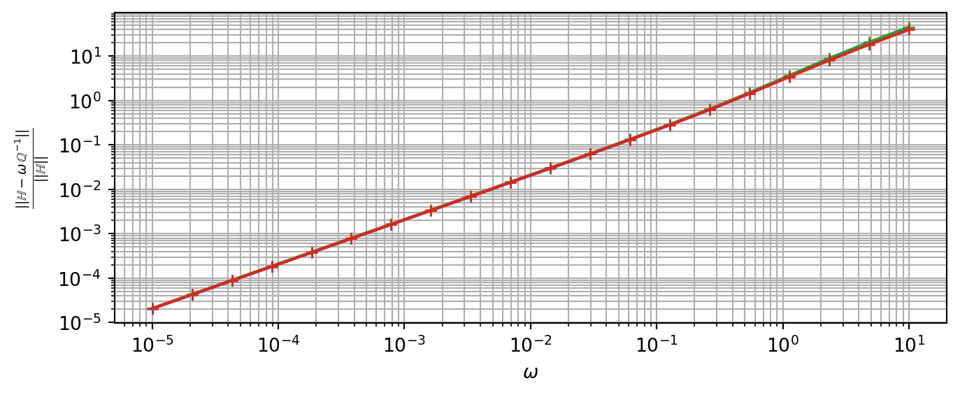
Linear spring interface model
In the fully open crack model considered so far, the two crack faces are traction-free. A more general model allows the faces to interact through a linear spring interface: the traction \(\uv{T}=\uu{\sig}\cdot\uv{n}\) on the crack face is linearly related to the displacement jump \(\jump{\uv{u}}\):
\[ \uv{T} = \left(k_n\,\uv{n}\otimes\uv{n} + k_t\,(\uu{1}-\uv{n}\otimes\uv{n})\right)\cdot\jump{\uv{u}} \tag{6.2}\]
where \(k_n \geq 0\) is the normal spring stiffness and \(k_t \geq 0\) the tangential one. The open crack (\(k_n=k_t=0\)) and the perfectly bonded interface (\(k_n,k_t\to\infty\)) are limiting cases.
Implementation
The spring stiffnesses are passed to the crack constructor via interf_prop (details in Chapter 14):
ver["CRACK"] = crack(shape=spheroidal(ω), density=d,
                     interf_prop={"C": [kn, kt]})
The order of parameters is [kn, kt] (normal first, tangential second). Passing prop={"C": tZ4} with no interf_prop is equivalent to the open crack (\(k_n=k_t=0\)).
Conductivity crack resistivity
The proper transport analog of the elastic crack compliance tensor is the crack resistivity tensor \(\uu{H}\) (Kachanov and Sevostianov, 2018). By analogy with the elastic case, it is defined from the 2nd-order second Hill tensor \(\uu{Q}=\uu{K}-\uu{K}\cdot\uu{P}\cdot\uu{K}\) as:
\[ \uu{H} = \lim_{\omega\to 0}\,\omega\,\uu{Q}^{-1} \tag{6.3}\]
The result is a positive semi-definite 3×3 tensor (rank-1 for an isotropic matrix, since only the normal component of the flux can jump across a crack).
WarningTerminology in Echoes
Although the physically correct term for the transport analog is crack resistivity, the function crack_compliance is used for both elasticity and transport in Echoes by analogy: passing a 2nd-order tensor K as the second argument automatically returns the 3×3 crack resistivity tensor \(\uu{H}\).
API
crack_compliance(shape, K) with a 2nd-order tensor K returns a 3×3 numpy.ndarray. As for the elastic case, \(\uu{H}\) does not depend on the aspect ratio \(\omega\) when \(\omega\to 0\), so only a small value needs to be provided.
For a spring-interface crack in conductivity, interf_prop={"K": [Ka, Kb, Kc]} sets the conductance along the three local axes of the crack (the two tangential axes first, then the normal):
ver["CRACK"] = crack(shape=spheroidal(ω), density=d,
                     interf_prop={"K": [Kt1, Kt2, Kn]})
For a spheroidal crack with rotational symmetry, \(K_{t1}=K_{t2}=K_t\) so the call reduces to [Kt, Kt, Kn].
Isotropic matrix
K_val = 2.5
K_iso = K_val * tId2

H_cond = crack_compliance(spheroidal(1.e-4), K_iso)
print("H (crack resistivity, isotropic) =\n", H_cond)

# Analytical formula: H_n = 2/(πK)  (n = e3, index 2)
H_n_formula = 2.0 / (math.pi * K_val)
print(f"\nFormula H[2,2] = 2/(πK) = {H_n_formula:.8f}")
print(f"Echoes  H[2,2]          = {H_cond[2,2]:.8f}")
print(f"Error:                    {abs(H_cond[2,2] - H_n_formula):.2e}")
H (crack resistivity, isotropic) =
[[0. 0. 0. ]
[0. 0. 0. ]
[0. 0. 0.25464791]]
Formula H[2,2] = 2/(πK) = 0.25464791
Echoes H[2,2] = 0.25464791
Error: 0.00e+00Anisotropic matrix
Just as for the 2nd-order Hill tensor (see Section 5.5), the crack resistivity is computed analytically for any matrix anisotropy.
# Orthotropic conductivity
K_aniso = tensor([3.2, 0.5, 1./(3.2*0.5)], angles=[math.pi/3, math.pi/4, math.pi/5])

H_aniso = crack_compliance(spheroidal(1.e-4), K_aniso)
print("H (crack resistivity, orthotropic) =\n", H_aniso)
H (crack resistivity, orthotropic) =
[[0. 0. 0. ]
[0. 0. 0. ]
[0. 0. 0.5368878]]\(\,\)