import numpy as np
from echoes import *
import math

np.set_printoptions(precision=8, suppress=True)
# to display only 8 significant digits of array components7 Ellipsoids
The Eshelby inhomogeneity problem (Eshelby, 1957)
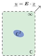
As in the inclusion problem presented in Chapter 5, the studied domain \(\Omega\) is the whole \(\R^3\) space. An ellipsoidal subdomain is still defined by \(\uv{x}\cdot(\trans{\uu{A}}\cdot\uu{A})^{-1}\cdot\uv{x}\leq 1\).
The material still obeys a linear elastic behavior with a uniform stiffness tensor \(\uuuu{C}\) outside the ellipsoid but now the material filling the ellipsoid is characterized by another stiffness tensor \(\uuuu{C}^\mathcal{I}\) without any polarization. This situation somehow corresponds to a fictitious polarization such that
\[ \sig(\x)=\uuuu{C}:\eps(\x)+\uu{\tau}(\x)\quad\textrm{where}\quad \uu{\tau}(\x)= \left\{ \begin{array}{ll} \uu{0}&\textrm{ if }\x \notin \mathcal{E}_{\uu{A}}\\ \left(\uuuu{C}^\mathcal{I}-\uuuu{C}\right):\eps(\x)=\delta\uuuu{C}:\eps(\x) &\textrm{ if }\x \in \mathcal{E}_{\uu{A}} \end{array} \right. \tag{7.1}\]
In addition the displacement is now of the form \(\E\cdot\x\) at infinity (i.e. remote homogeneous strain condition such that the problem solution would be \(\eps=\E\) if the ellipsoid and the matrix shared the same elasticity).
The second important result derived in (Eshelby, 1957) is that the strain tensor field solution to this problem is also uniform within the ellipsoidal domain (not outside!) and writes
\[ \forall \x \in \mathcal{E}_{\uu{A}},\quad \eps(\x)=\uuuu{A}^E:\E \quad\textrm{ where } \uuuu{A}^E=\left(\uuuu{I}+\uuuu{P}:\delta\uuuu{C}\right)^{-1} \tag{7.2}\]
\(\uuuu{A}^E\) is called the strain-strain concentration tensor for the Eshelby problem and \(\uuuu{P}(\uu{A},\uuuu{C})\) is the Hill polarization tensor already introduced in Chapter 5, depending only on the shape and orientation of the ellipsoid \(\uu{A}\) and the matrix behavior \(\uuuu{C}\), not on that of the ellipsoidal inhomogeneity \(\uuuu{C}^\mathcal{I}\).
Ellipsoidal inhomogeneity in Echoes
An inhomogeneity of ellipsoidal shape is built in Echoes by
ell = ellipsoid(shape=..., prop={"C":..., "D":...})Such an ellipsoid object is defined by a shape (either ellipsoidal, spheroidal or spherical as presented in Section 5.2) and a dictionary of properties of names arbitrarily chosen by the user.
It is possible to change the shape and prop values after construction:
ell.shape = spheroidal(0.1, math.pi/3, math.pi/4)
ell.set_prop("C", stiff_kmu(3., 2.))
In order to simulate the Eshelby problem so as to calculate the concentration tensor \(\uuuu{A}^E\), it is necessary to define the reference medium in which the ellipsoid is embedded. This is done by
C = ...
ell.set_ref("C", C)
WarningWarning
The tensor introduced in set_ref must not be built on the fly, i.e. it must be built before using in set_ref and not destroyed before calculating concentration tensors. Moreover set_ref must be applied each time the ellipsoid is modified (by shape or set_prop).
Once the reference medium is set for the desired property, the strain-strain concentration tensor is obtained by
ell.eE
NoteNotes
- The terminology
eErecalls that this concentration tensor relates the microscopic strain (efor epsilon) to the macroscopic strain (Efor \(\E\)). - The object returned is not a
tensor(which is designed only for symmetric tensors) but a \(6\times 6\)numpy.ndarraysince \(\uuuu{A}^E\) may not fulfill the major symmetry (i.e. not necessarily symmetric in its Kelvin-Mandel notation). - The Hill tensor required in the concentration tensor is calculated with default parameters (analytical if the matrix is isotropic, using the
NUMINTalgorithm if the matrix is anisotropic). However it is possible to force parameters by applyingell.set_param_eshelby(algo=NUMINT, epsroots=1.e-4, epsabs=1.e-4, epsrel=1.e-4, maxnb=100000).
ell = ellipsoid(shape=spherical, prop={"C": stiff_kmu(5., 3.)})
C = stiff_kmu(72., 32.)
for ω in [0.1, 1.]:
    ell.shape = spheroidal(ω)
    ell.set_ref("C", C)
    A = ell.eE
    print(f"AE(ω={ω})=\n", A, "\n")
    # note that A is not major-symmetric if ω≠1
AE(ω=0.1)=
[[ 1.09739726 -0.01470205 -0.09705466 0. 0. 0. ]
[-0.01470205 1.09739726 -0.09705466 0. 0. 0. ]
[ 2.72334206 2.72334206 7.43195797 0. 0. 0. ]
[ 0. 0. 0. 4.21367365 0. 0. ]
[ 0. 0. 0. 0. 4.21367365 0. ]
[ 0. 0. 0. 0. 0. 1.11209931]]
AE(ω=1.0)=
[[1.97133616 0.21712912 0.21712912 0. 0. 0. ]
[0.21712912 1.97133616 0.21712912 0. 0. 0. ]
[0.21712912 0.21712912 1.97133616 0. 0. 0. ]
[0. 0. 0. 1.75420704 0. 0. ]
[0. 0. 0. 0. 1.75420704 0. ]
[0. 0. 0. 0. 0. 1.75420704]]
ell.shape = spheroidal(0.1, math.pi/3, math.pi/4)
ell.set_prop("C", stiff_kmu(3., 2.))
ell.set_ref("C", C)
print(ell)
print(ell.eE)
Ellipsoid | Volume fraction=0 | Radii=[1 1 0.1] | Angles=[1.0472 0.785398 0]
Parameters for Eshelby calculation=[ DEFAULT ; epsabs=0.0001 ; epsrel=0.0001 ; epsroots=0.0001 ]
--> Property C
Order 4 ISO tensor | Param(size=2)=[ 9 4 ] | Angles(size=0)=[ ]
[ 5.66667 1.66667 1.66667 0 0 0
1.66667 5.66667 1.66667 0 0 0
1.66667 1.66667 5.66667 0 0 0
0 0 0 4 0 0
0 0 0 0 4 0
0 0 0 0 0 4 ]
[[ 4.75034232 0.91713011 1.04575424 -0.44556704 1.12297667 1.37535992]
[ 0.91713011 4.75034232 1.04575424 1.12297667 -0.44556704 1.37535992]
[ 0.58974478 0.58974478 3.60732982 1.2568717 1.2568717 -0.38171871]
[ 1.13409604 2.70263975 2.83653478 2.91658667 0.89457273 0.54105942]
[ 2.70263975 1.13409604 2.83653478 0.89457273 2.91658667 0.54105942]
[ 3.31004418 3.31004418 1.55296555 0.54105942 0.54105942 3.13747326]]The four concentration tensors
Observing that \(\sig=\uuuu{C}^\mathcal{I}:\eps\) within the ellipsoid and introducing the macroscopic stress tensor \(\Sig=\uuuu{C}:\E\), all concentration tensors can be defined as
\[ \begin{aligned} \eps_{|\mathcal{E}_{\uu{A}}}=\uuuu{A}^E:\E&&\\ \eps_{|\mathcal{E}_{\uu{A}}}=\uuuu{A}^\Sigma:\Sig&\quad\textrm{ with }\quad \uuuu{A}^\Sigma=\uuuu{A}^E:\uuuu{C}^{-1}&\\ \sig_{|\mathcal{E}_{\uu{A}}}=\uuuu{B}^E:\E&\quad\textrm{ with }\quad \uuuu{B}^E=\uuuu{C}^\mathcal{I}:\uuuu{A}^E&\\ \sig_{|\mathcal{E}_{\uu{A}}}=\uuuu{B}^\Sigma:\Sig&\quad\textrm{ with }\quad \uuuu{B}^\Sigma=\uuuu{C}^\mathcal{I}:\uuuu{A}^E:\uuuu{C}^{-1}& \end{aligned} \tag{7.3}\]
These concentration tensors are accessible through the attributes eE, eS, sE and sS.
ell = ellipsoid(shape=spherical, prop={"C": stiff_kmu(5., 3.)})
C = stiff_kmu(72., 32.)
for ω in [0.1, 1.]:
    ell.shape = spheroidal(ω)
    ell.set_ref("C", C)
    print(f"AE(ω={ω})=\n", ell.eE, "\n")
    print(f"AS(ω={ω})=\n", ell.eS, "\n")
    print(f"BE(ω={ω})=\n", ell.sE, "\n")
    print(f"BS(ω={ω})=\n", ell.sS, "\n")
AE(ω=0.1)=
[[ 1.09739726 -0.01470205 -0.09705466 0. 0. 0. ]
[-0.01470205 1.09739726 -0.09705466 0. 0. 0. ]
[ 2.72334206 2.72334206 7.43195797 0. 0. 0. ]
[ 0. 0. 0. 4.21367365 0. 0. ]
[ 0. 0. 0. 0. 4.21367365 0. ]
[ 0. 0. 0. 0. 0. 1.11209931]]
AS(ω=0.1)=
[[ 0.01353434 -0.00384221 -0.00512897 0. 0. 0. ]
[-0.00384221 0.01353434 -0.00512897 0. 0. 0. ]
[-0.00464959 -0.00464959 0.06892253 0. 0. 0. ]
[ 0. 0. 0. 0.06583865 0. 0. ]
[ 0. 0. 0. 0. 0.06583865 0. ]
[ 0. 0. 0. 0. 0. 0.01737655]]
BE(ω=0.1)=
[[18.00249537 11.32989949 21.13121804 0. 0. 0. ]
[11.32989949 18.00249537 21.13121804 0. 0. 0. ]
[27.75816418 27.75816418 66.30529382 0. 0. 0. ]
[ 0. 0. 0. 25.28204193 0. 0. ]
[ 0. 0. 0. 0. 25.28204193 0. ]
[ 0. 0. 0. 0. 0. 6.67259588]]
BS(ω=0.1)=
[[ 0.09633362 -0.00792569 0.14521991 0. 0. 0. ]
[-0.00792569 0.09633362 0.14521991 0. 0. 0. ]
[-0.01276997 -0.01276997 0.58952893 0. 0. 0. ]
[ 0. 0. 0. 0.39503191 0. 0. ]
[ 0. 0. 0. 0. 0.39503191 0. ]
[ 0. 0. 0. 0. 0. 0.10425931]]
AE(ω=1.0)=
[[1.97133616 0.21712912 0.21712912 0. 0. 0. ]
[0.21712912 1.97133616 0.21712912 0. 0. 0. ]
[0.21712912 0.21712912 1.97133616 0. 0. 0. ]
[0. 0. 0. 1.75420704 0. 0. ]
[0. 0. 0. 0. 1.75420704 0. ]
[0. 0. 0. 0. 0. 1.75420704]]
AS(ω=1.0)=
[[ 0.02198533 -0.00542416 -0.00542416 0. 0. 0. ]
[-0.00542416 0.02198533 -0.00542416 0. 0. 0. ]
[-0.00542416 -0.00542416 0.02198533 0. 0. 0. ]
[ 0. 0. 0. 0.02740948 0. 0. ]
[ 0. 0. 0. 0. 0.02740948 0. ]
[ 0. 0. 0. 0. 0. 0.02740948]]
BE(ω=1.0)=
[[19.04480018 8.51955795 8.51955795 0. 0. 0. ]
[ 8.51955795 19.04480018 8.51955795 0. 0. 0. ]
[ 8.51955795 8.51955795 19.04480018 0. 0. 0. ]
[ 0. 0. 0. 10.52524222 0. 0. ]
[ 0. 0. 0. 0. 10.52524222 0. ]
[ 0. 0. 0. 0. 0. 10.52524222]]
BS(ω=1.0)=
[[0.165323 0.00086609 0.00086609 0. 0. 0. ]
[0.00086609 0.165323 0.00086609 0. 0. 0. ]
[0.00086609 0.00086609 0.165323 0. 0. 0. ]
[0. 0. 0. 0.16445691 0. 0. ]
[0. 0. 0. 0. 0.16445691 0. ]
[0. 0. 0. 0. 0. 0.16445691]]
\(\,\)