import numpy as np
from echoes import *
import math
import matplotlib.pyplot as plt

np.set_printoptions(precision=8, suppress=True)13 Homogenization of porous media
Porous medium modeling
A porous medium is modeled as a composite in which the voids are treated as inclusions with zero (or near-zero) stiffness:
ks, mus = 72., 32.
kp, mup = 1.e-6, 1.e-6

myrve = rve(matrix="SOLID")
myrve["SOLID"] = ellipsoid(shape=spheroidal(1.), symmetrize=[ISO],
                           prop={"C": stiff_kmu(ks, mus)})
myrve["PORE"] = ellipsoid(shape=spheroidal(1.), symmetrize=[ISO],
                          prop={"C": stiff_kmu(kp, mup)})
Scheme comparison on porous media
The following example computes the effective bulk and shear moduli versus porosity for all available schemes.
Figure — scheme comparison on porous media
def Chom_porous(myrve, phi, sch):
    myrve["PORE"].fraction = phi
    myrve["SOLID"].fraction = 1. - phi
    try:
        C = homogenize(prop="C", rve=myrve, scheme=sch,
                       verbose=False, epsrel=1.e-6, maxnb=300,
                       select_best=True)
        return max(C.k, 0.), max(C.mu, 0.)
    except:
        return 0., 0.

lphi = np.linspace(0., 1., 51)

fig, (ax1, ax2) = plt.subplots(1, 2, figsize=(9, 4))
for sch in [VOIGT, REUSS, DIL, MT, SC, DIFF, PCW, MAX]:
    lk, lmu = [], []
    for phi in lphi:
        k, mu = Chom_porous(myrve, phi, sch)
        lk.append(k)
        lmu.append(mu)
    ax1.plot(lphi, lk, label=str(sch))
    ax2.plot(lphi, lmu, label=str(sch))

ax1.set_xlabel(r"$\varphi$"); ax1.set_ylabel(r"$k^{hom}$")
ax1.grid(True); ax1.legend()
ax2.set_xlabel(r"$\varphi$"); ax2.set_ylabel(r"$\mu^{hom}$")
ax2.grid(True); ax2.legend()
plt.tight_layout()
plt.show()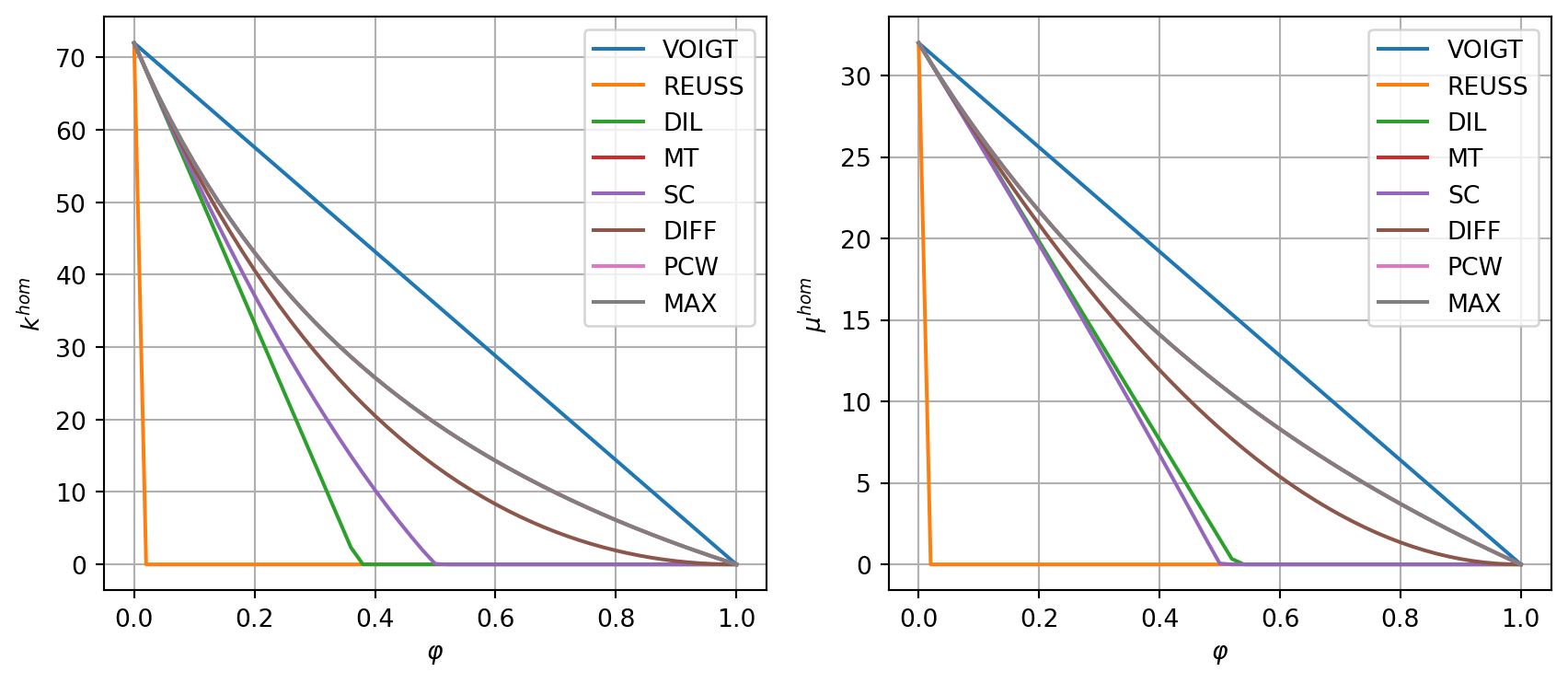
Effect of pore shape
The aspect ratio of pores significantly affects the effective properties. Both oblate (\(\omega < 1\)) and prolate (\(\omega > 1\)) pores lead to softer behavior than spherical pores (\(\omega = 1\)), i.e. the effective moduli decrease more rapidly with porosity.
Figure — effect of pore shape
lphi = np.linspace(0., 0.5, 51)
fig, (ax1, ax2) = plt.subplots(1, 2, figsize=(9, 4))

for omega, style in [(0.1, '--'), (1., '-'), (10., ':')]:
    myrve["PORE"].shape = spheroidal(omega)
    myrve["SOLID"].shape = spheroidal(1.)
    lk, lmu = [], []
    for phi in lphi:
        k, mu = Chom_porous(myrve, phi, SC)
        lk.append(k)
        lmu.append(mu)
    ax1.plot(lphi, lk, style, label=f"SC, ω={omega}")
    ax2.plot(lphi, lmu, style, label=f"SC, ω={omega}")

ax1.set_xlabel(r"$\varphi$"); ax1.set_ylabel(r"$k^{hom}$")
ax1.grid(True); ax1.legend()
ax2.set_xlabel(r"$\varphi$"); ax2.set_ylabel(r"$\mu^{hom}$")
ax2.grid(True); ax2.legend()
plt.tight_layout()
plt.show()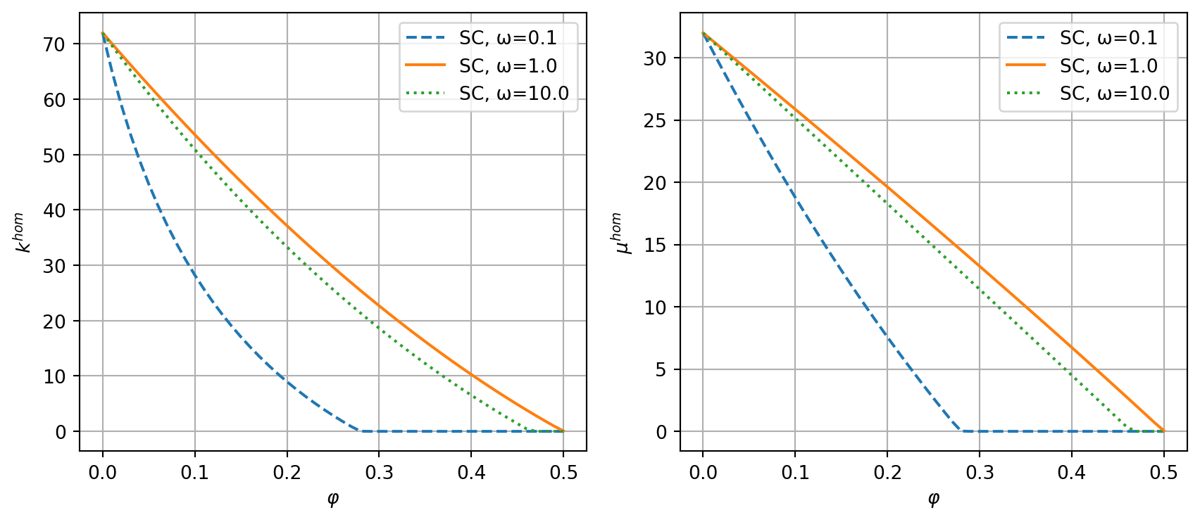
Percolation threshold
In the self-consistent scheme, the effective moduli vanish at a critical porosity (percolation threshold) that depends on the pore aspect ratio. For spherical pores (\(\omega=1\)), the percolation threshold is \(\phi_c=0.5\). Both flattening (\(\omega < 1\)) and elongating (\(\omega > 1\)) the pores lower the percolation threshold below \(0.5\): non-spherical pores create more connectivity at a given volume fraction, so the medium loses its stiffness earlier.
Permeability of porous media
Transport properties (permeability, conductivity, diffusivity) are described by 2nd-order tensors and can be homogenized with the same framework using prop="K":
Figure — permeability of a porous medium
Ks = 0.1 * tId2    # solid conductivity
Kp = tId2           # pore conductivity

myrve_K = rve(matrix="SOLID")
myrve_K["SOLID"] = ellipsoid(shape=spheroidal(1.), symmetrize=[ISO],
                             prop={"K": Ks})
myrve_K["PORE"] = ellipsoid(shape=spheroidal(0.1), symmetrize=[ISO],
                            prop={"K": Kp})

lphi = np.linspace(0., 0.7, 51)
fig, ax = plt.subplots(figsize=(6, 5))
for sch in [MT, SC, MAX]:
    lK = []
    for phi in lphi:
        myrve_K["PORE"].fraction = phi
        myrve_K["SOLID"].fraction = 1. - phi
        try:
            K = homogenize(prop="K", rve=myrve_K, scheme=sch,
                           verbose=False, maxnb=300, epsrel=1.e-10,
                           select_best=True)
            lK.append(max(np.trace(K.array) / 3., 0.))
        except:
            lK.append(0.)
    ax.plot(lphi, lK, label=str(sch))

ax.set_xlabel(r"$\varphi$"); ax.set_ylabel(r"$K^{hom}$")
ax.set_ylim(0., 1.)
ax.grid(True); ax.legend()
plt.show()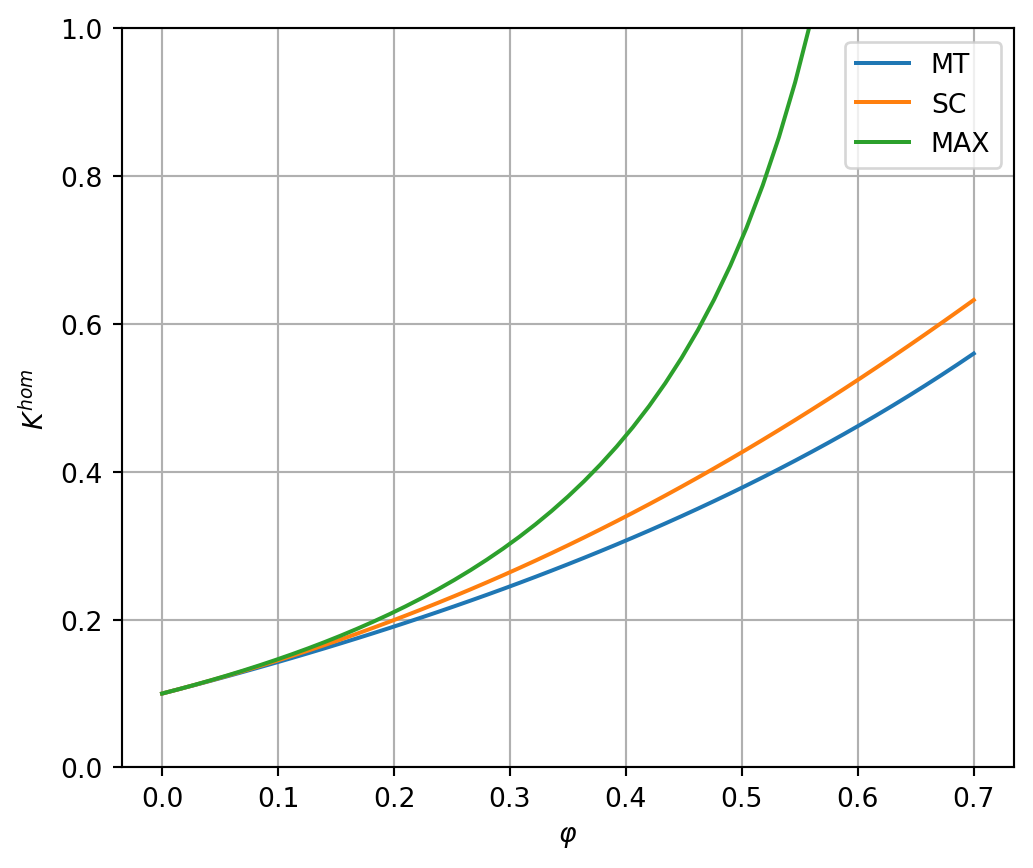
\(\,\)