import numpy as np
from echoes import *
import math

np.set_printoptions(precision=8, suppress=True)14 Homogenization of cracked media
Isotropic randomly cracked medium
For randomly oriented penny-shaped cracks in an isotropic matrix, the symmetrize=[ISO] option projects the concentration tensor onto the isotropic symmetry class. This yields scalar effective bulk and shear moduli.
Figure — effective moduli of a randomly cracked isotropic medium
import matplotlib.pyplot as plt

ω = 1.e-3
Cs = stiff_Enu(1., 0.2)   # matrix: E=1, ν=0.2

myrve = rve(matrix="SOLID")
myrve["SOLID"] = ellipsoid(shape=spherical, fraction=1.,
                            prop={"C": Cs, "K": 1. * tId2})
myrve["CRACK"] = crack(shape=spheroidal(ω), symmetrize=[ISO],
                        prop={"C": tZ4, "K": tensor(ω, ω, 1.)})

ld = np.linspace(0., 1.2, 61)
fig, axes = plt.subplots(1, 2, figsize=(9, 4))

for sch, ls in zip([MT, SC, ASC, MAX, DIFF, PCW],
                   ['-', '-', '--', '--', '-.', ':']):
    lk, lmu = [], []
    for d in ld:
        myrve["CRACK"].density = d
        myrve.set_prop("C", Cs)
        try:
            C = homogenize(prop="C", rve=myrve, scheme=sch,
                           verbose=False, epsrel=1.e-6, maxnb=300,
                           select_best=True)
            lk.append(max(C.k / Cs.k, 0.))
            lmu.append(max(C.mu / Cs.mu, 0.))
        except Exception:
            lk.append(0.)
            lmu.append(0.)
    axes[0].plot(ld, lk, ls, label=str(sch))
    axes[1].plot(ld, lmu, ls, label=str(sch))

for ax, lbl in zip(axes, [r"$k^{hom}/k^s$", r"$\mu^{hom}/\mu^s$"]):
    ax.set_xlabel(r"$\varepsilon$")
    ax.set_ylabel(lbl)
    ax.set_ylim(0., 1.05)
    ax.grid(True)
    ax.legend(loc="best", fontsize=8)
plt.tight_layout()
plt.show()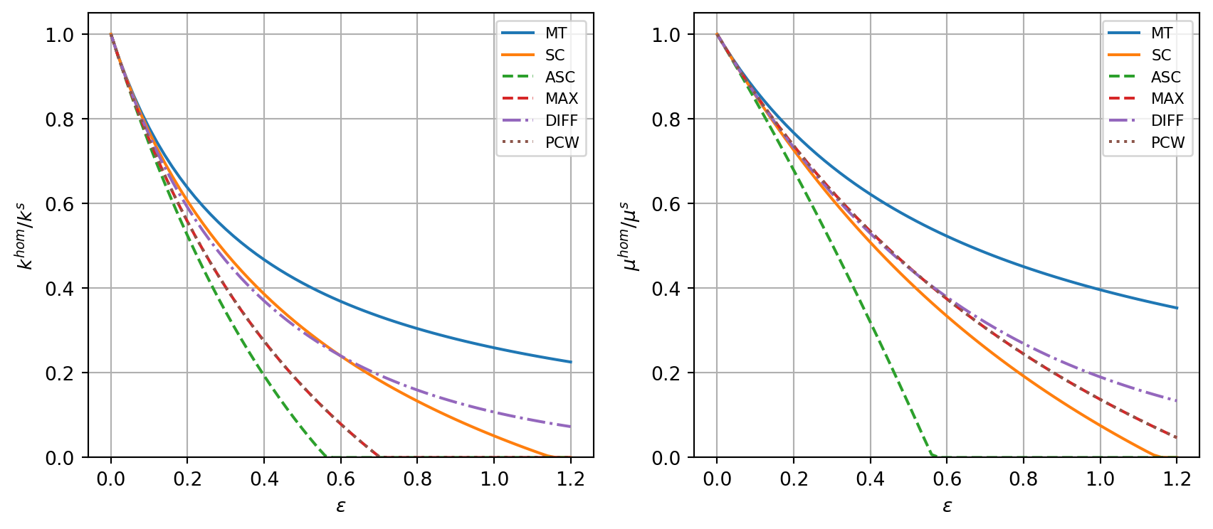
Transversely isotropic crack distribution
When crack normals are not fully random but distributed with TI symmetry around an axis, symmetrize=[TI, θ, φ] is used instead of [ISO]. A representative case is that of cracks whose normals lie uniformly in a plane — obtained by taking a single crack orientation and averaging over rotations around the perpendicular axis.
The example below uses ellipsoidal(1., ω, 1./ω) — a crack thin in \(\uv{e}_2\) (normal \(= \uv{e}_2\)) and elongated in \(\uv{e}_3\). symmetrize=[TI, 0., 0.] then averages over rotations around \(\uv{e}_3\), sweeping crack normals through the \((\uv{e}_1,\uv{e}_2)\) plane. The resulting effective medium is TI with axis \(\uv{e}_3\): the in-plane stiffness \(C_{1111}\) is strongly degraded while the longitudinal conductivity \(K_{11}\) is enhanced by the high normal conductance \(K_n \gg 1\) of the cracks.
Figure — TI crack distribution: stiffness and conductivity
ω = 1.e-4 ; ko = 1.e-10 ; Kt = 1. ; Kn = 1.e10
Cs = stiff_Enu(1., 0.2)
C11s = Cs.array[0, 0]

myrve_ti = rve(matrix="SOLID")
myrve_ti["SOLID"] = ellipsoid(shape=spherical, fraction=1.,
                               prop={"C": Cs, "K": ko * tId2})
# Crack: normal along e2 (thin dimension), elongated in e3
# TI averaging around e3 → normals sweep (e1,e2) plane
myrve_ti["CRACK"] = crack(shape=ellipsoidal(1., ω, 1./ω, 0., 0., 0.),
                           symmetrize=[TI, 0., 0.],
                           prop={"C": tZ4, "K": tensor(Kt, Kn, Kt)})

ld = np.linspace(0., 0.8, 101)
fig, axes = plt.subplots(1, 2, figsize=(9, 4))

for sch, ls in zip([MT, SC, DIFF], ['-', '-', '--']):
    lC11, lK11 = [], []
    for d in ld:
        myrve_ti["CRACK"].density = d
        myrve_ti.set_prop("C", Cs)
        try:
            C = homogenize(prop="C", rve=myrve_ti, scheme=sch,
                           verbose=False, epsrel=1.e-6, maxnb=100,
                           select_best=True)
            val = C.array[0, 0] / C11s
            lC11.append(val if val > 0. else np.nan)
        except Exception:
            lC11.append(np.nan)
        myrve_ti.set_prop("K", ko * tId2)
        try:
            K = homogenize(prop="K", rve=myrve_ti, scheme=sch,
                           verbose=False, epsrel=1.e-6, maxnb=100,
                           select_best=True)
            lK11.append(K.array[0, 0] / (ω * Kt))
        except Exception:
            lK11.append(np.nan)
    axes[0].plot(ld, lC11, ls, label=str(sch))
    axes[1].plot(ld, lK11, ls, label=str(sch))

axes[0].set_xlabel(r"$\varepsilon$"); axes[0].set_ylabel(r"$C^{hom}_{1111}/C^s_{1111}$")
axes[0].set_ylim(0., 1.05); axes[0].grid(True); axes[0].legend(fontsize=8)
axes[1].set_xlabel(r"$\varepsilon$"); axes[1].set_ylabel(r"$K^{hom}_{11}/(\omega K_t)$")
axes[1].grid(True); axes[1].legend(fontsize=8)
plt.tight_layout()
plt.show()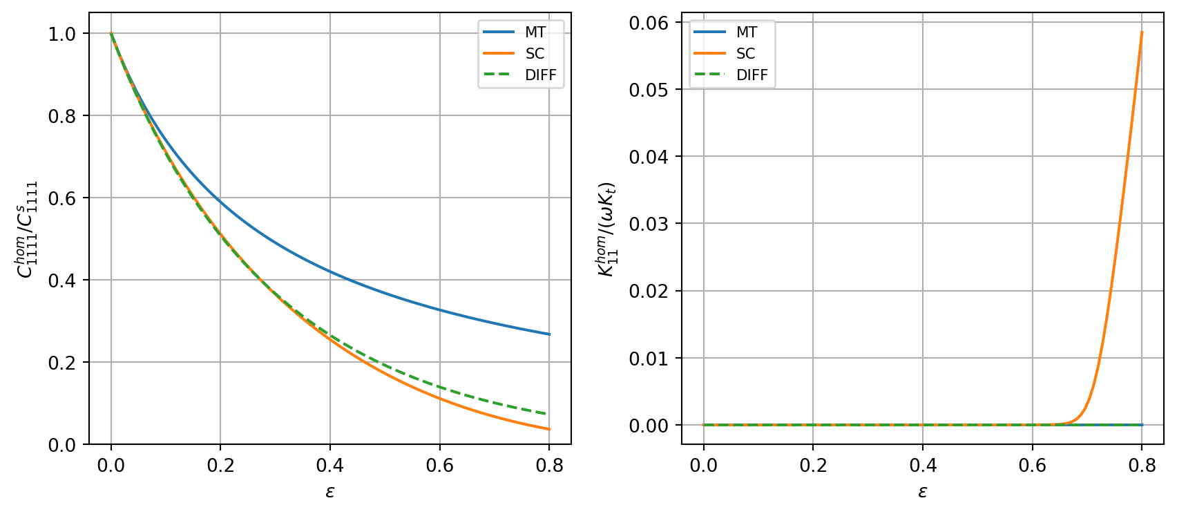
Spring interface model
The open crack (\(k_n=k_t=0\)) is a limiting case. When the crack faces are partially bonded, the linear spring model from Section 6.3 is activated via interf_prop. For elasticity the parameter order is [kn, kt]:
Spring interface model — open / bonded limits
Cs = stiff_Enu(1., 0.2)
myrve_spr = rve(matrix="SOLID")
myrve_spr["SOLID"] = ellipsoid(shape=spherical, fraction=1., prop={"C": Cs})
myrve_spr["CRACK"] = crack(shape=spheroidal(1.e-3), density=0.3,
                            symmetrize=[ISO], prop={"C": tZ4})

C_open   = homogenize(prop="C", rve=myrve_spr, scheme=MT)

myrve_spr["CRACK"].set_interf_prop("C", [5., 5.])
C_spring = homogenize(prop="C", rve=myrve_spr, scheme=MT)

myrve_spr["CRACK"].set_interf_prop("C", [1.e12, 1.e12])
C_bonded = homogenize(prop="C", rve=myrve_spr, scheme=MT)

print(f"E (matrix solid)     = {Cs.E:.6f}")
print(f"E (open crack)       = {C_open.E:.6f}")
print(f"E (spring kn=kt=5)   = {C_spring.E:.6f}")
print(f"E (perfect bonding)  = {C_bonded.E:.6f}")
E (matrix solid) = 1.000000
E (open crack) = 0.651284
E (spring kn=kt=5) = 0.947176
E (perfect bonding) = 1.000588Randomly cracked medium: coupled elasticity and conductivity
Cracks significantly affect both the mechanical and transport properties of the medium. The crack object accepts both prop={"C": ..., "K": ...} (material properties of the crack medium) and interf_prop={"C": [kn, kt], "K": [Ka, Kb, Kc]} (interface stiffnesses). For elasticity [kn, kt] means normal then tangential stiffness. For conductivity [Ka, Kb, Kc] are the conductances along the three local crack axes (the two tangential axes first, then the normal): for a spheroidal crack, [Kt, Kt, Kn]. For a void crack with high conductivity across the crack plane, typical settings are prop={"C": tZ4, "K": tensor(Kt, Kt, Kn)} where Kn is large.
Figure — cracked medium: coupled Young’s modulus and conductivity
ω = 1.e-3 ; ko = 1. ; kt_K = 1.e9   # high conductance (fluid-filled crack)

Cs = stiff_Enu(1., 0.25)

myrve_al = rve(matrix="SOLID")
myrve_al["SOLID"] = ellipsoid(shape=spherical, fraction=1.,
                               prop={"C": Cs, "K": ko * tId2})
myrve_al["CRACK"] = crack(shape=spheroidal(ω), symmetrize=[ISO],
                           prop={"C": tZ4, "K": tensor(kt_K, kt_K, kt_K)})

ld = np.linspace(0., 1.2, 61)
fig, axes = plt.subplots(1, 2, figsize=(9, 4))

for sch, ls in zip([MT, SC, ASC, DIFF, PCW],
                   ['-', '-', '--', '-.', ':']):
    lE, lK = [], []
    pcw_zeroed = False
    for d in ld:
        myrve_al["CRACK"].density = d
        myrve_al.set_prop("C", Cs)
        if sch is PCW and pcw_zeroed:
            lE.append(np.nan)
        else:
            try:
                C = homogenize(prop="C", rve=myrve_al, scheme=sch,
                               verbose=False, epsrel=1.e-5, maxnb=200,
                               select_best=True)
                val = C.E / Cs.E
                if val <= 0.:
                    lE.append(np.nan)
                    if sch is PCW:
                        pcw_zeroed = True
                else:
                    lE.append(val)
            except Exception:
                lE.append(np.nan)
        myrve_al.set_prop("K", ko * tId2)
        try:
            K = homogenize(prop="K", rve=myrve_al, scheme=sch,
                           verbose=False, epsrel=1.e-5, maxnb=200,
                           select_best=True)
            val = K.param[0] / ko
            lK.append(val if val > 0. else np.nan)
        except Exception:
            lK.append(np.nan)
    axes[0].plot(ld, lE, ls, label=str(sch))
    axes[1].plot(ld, lK, ls, label=str(sch))

axes[0].set_xlabel(r"$\varepsilon$"); axes[0].set_ylabel(r"$E^{hom}/E^s$")
axes[0].set_ylim(0., 1.05); axes[0].grid(True); axes[0].legend(fontsize=8)
axes[1].set_xlabel(r"$\varepsilon$"); axes[1].set_ylabel(r"$K^{hom}/K^s$")
axes[1].grid(True); axes[1].legend(fontsize=8)
plt.tight_layout()
plt.show()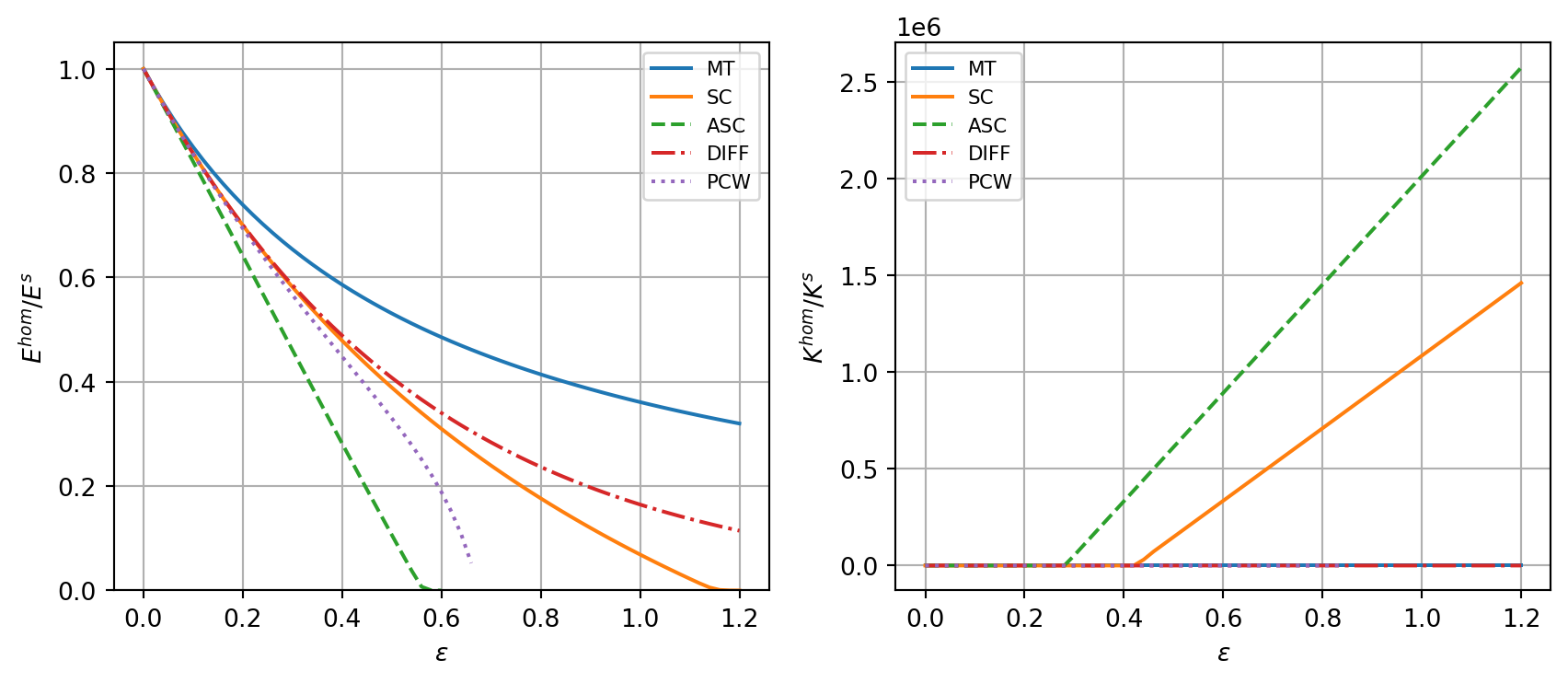
Multiple crack families
Several crack families with different orientations and properties can be assembled in one RVE. The example below considers two families of cracks with different orientations and finite conductivity, computing the effective stiffness and permeability simultaneously:
Multiple crack families — stiffness and permeability
π = math.pi
ko = 1.e-10 ; kinf = 1.e10

myrve2 = rve(matrix="SOLID")
myrve2["SOLID"] = ellipsoid(shape=spherical, fraction=1,
    prop={"K": ko * tId2, "C": stiff_kmu(1., 1.)})
myrve2["CRACK1"] = crack(shape=spheroidal(1.e-3, π/3., π/5.), density=0.4,
    prop={"C": tZ4}, interf_prop={"K": [2., 2., kinf]})
myrve2["CRACK2"] = crack(shape=spheroidal(1.e-3, π/6.), density=0.3,
    prop={"C": tZ4}, interf_prop={"K": [2., 2., kinf]})

C_eff = homogenize(prop="C", rve=myrve2, scheme=SC,
                   verbose=False, epsrel=1.e-6, maxnb=200)
print("Effective stiffness:\n", C_eff)

K_eff = homogenize(prop="K", rve=myrve2, scheme=SC,
                   verbose=False, epsrel=1.e-6, maxnb=200)
print("\nEffective permeability:\n", K_eff)
Effective stiffness:
Order 4 ORTHO tensor | Param(size=9)=[ 1.30624 0.168788 0.0440703 2.27612 0.0401982 0.277515 0.348474 0.269905 0.773451 ] | Angles(size=3)=[ 0.812673 0.451506 0.59908 ]
[ 1.10574 0.187443 0.217777 0.127348 -0.582399 -0.413308
0.187443 1.4345 0.099249 -0.0912792 -0.0591347 -0.473671
0.217777 0.099249 0.816809 -0.0714946 -0.490448 -0.00777335
0.127348 -0.0912792 -0.0714946 0.985001 -0.200532 -0.397897
-0.582399 -0.0591347 -0.490448 -0.200532 1.05707 0.0898749
-0.413308 -0.473671 -0.00777335 -0.397897 0.0898749 1.24442 ]
Effective permeability:
Order 2 ORTHO tensor | Param(size=3)=[ 3.83052e-09 3.23741e-09 6.41501e-10 ] | Angles(size=3)=[ 0.803909 0.443179 5.31722 ]
[ 2.43722e-09 -7.62836e-10 -1.34399e-09
-7.62836e-10 3.18528e-09 -4.16817e-10
-1.34399e-09 -4.16817e-10 2.08693e-09 ]
\(\,\)