$$ \newcommand{\C}{{\mathbb{{C}}}} \newcommand{\R}{{\mathbb{{R}}}} \newcommand{\Q}{{\mathbb{{Q}}}} \newcommand{\Z}{{\mathbb{{Z}}}} \newcommand{\N}{{\mathbb{{N}}}} \newcommand{\uu}[1]{{\boldsymbol{{#1}}}} \newcommand{\uuuu}[1]{{\symbb{{#1}}}} \newcommand{\uv}[1]{{\underline{{#1}}}} \newcommand{\ve}[1]{{\uv{{e}}_{{#1}}}} \newcommand{\x}{{\uv{{x}}}} \newcommand{\n}{{\uv{{n}}}} \newcommand{\eps}{{\uu{{\varepsilon}}}} \newcommand{\E}{{\uu{{E}}}} \newcommand{\sig}{{\uu{{\sigma}}}} \newcommand{\Sig}{{\uu{{\Sigma}}}} \newcommand{\cod}{{\uv{{\symscr{b}}}}} \newcommand{\trans}[1]{{{}^{t}{#1}}} \newcommand{\sotimes}{{\stackrel{s}{\otimes}}} \newcommand{\sboxtimes}{\stackrel{s}{\boxtimes}} \newcommand{\norm}[1]{{\lVert{{#1}}\rVert}} \newcommand{\ud}{{\,\mathrm{d}}} \newcommand{\mat}{\mathsf} \DeclareMathOperator{\arcosh}{arcosh} \DeclareMathOperator{\divz}{div} \DeclareMathOperator{\divu}{\uv{div}} \DeclareMathOperator{\hess}{hess} \DeclareMathOperator{\gradu}{\uv{grad}} \DeclareMathOperator{\graduu}{\uu{grad}} \DeclareMathOperator{\Mat}{Mat} \DeclareMathOperator{\tr}{tr} \DeclareMathOperator{\ISO}{ISO} \newcommand{\volt}[1]{{#1}^{-1\circ}} \newcommand{\dcirc}{\overset{\circ}{:}} \newcommand{\jump}[1]{\mathopen{[\![}\,#1\,\mathclose{]\!]}} $$

15 Exercises on homogenization schemes

Objectives

This tutorial provides hands-on exercises on homogenization schemes: porous medium with all schemes, the 3-phase model, a multiscale hierarchical structure, and parameter identification on sandstone.

Imports

import numpy as np
from echoes import *
import math
import matplotlib.pyplot as plt

np.set_printoptions(precision=8, suppress=True)

Exercise 1: Elasticity of a porous medium

Exercise

The objective is to plot the bulk and shear moduli of a porous medium as a function of porosity, comparing the schemes VOIGT, REUSS, DIL, MT, SC, and the 3-phase model.

The solid phase is isotropic with $k_s=72$ GPa and $\mu_s=32$ GPa. The pores are represented by a near-zero stiffness material ($k_p=10^{-6}$, $\mu_p=10^{-6}$).

Build a function buildrve(ws, wp) returning the rve in which the solid and pores are randomly distributed spheroids with respective aspect ratios ws and wp.
Build a function Chom(myrve, phi, sch) returning the tuple (khom, muhom). Handle non-physical negative values by replacing them with 0.
Plot $k^{hom}(\varphi)$ and $\mu^{hom}(\varphi)$ for all 5 schemes with spherical inclusions.
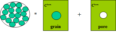
The 3-phase model consists in a self-consistent scheme with a single phase: a 2-layer sphere with a spherical pore as inner core (radius $\varphi^{1/3}$) surrounded by the solid. Build the corresponding rve3ph and function Chom3ph(phi).
Add the 3-phase model curve to the comparison plot.
Change the aspect ratios to examine their impact on the predictions.

Solution

Cs = stiff_kmu(72., 32.)
Cp = stiff_kmu(1.e-6, 1.e-6)

def buildrve(ws, wp):
    myrve = rve(matrix="SOLID")
    myrve["SOLID"] = ellipsoid(shape=spheroidal(ws), symmetrize=[ISO], prop={"C": Cs})
    myrve["PORE"]  = ellipsoid(shape=spheroidal(wp),  symmetrize=[ISO], prop={"C": Cp})
    return myrve

def Chom(myrve, phi, sch):
    myrve["PORE"].fraction  = phi
    myrve["SOLID"].fraction = 1. - phi
    C = homogenize(prop="C", rve=myrve, scheme=sch,
                   verbose=False, epsrel=1.e-10, maxnb=300, select_best=True)
    return max(C.k, 0.), max(C.mu, 0.)

# 3-phase model: SC with a single 2-layer sphere (pore core + solid shell)
rve3ph = rve(matrix="SPN")
rve3ph["SPN"] = sphere_nlayers(radii=[0.5, 1.], fraction=1., prop={"C": [Cp, Cs]})

def Chom3ph(phi):
    rve3ph["SPN"].set_radius(0, math.pow(phi, 1./3.))
    C = homogenize(prop="C", rve=rve3ph, scheme=SC, verbose=False)
    return max(C.k, 0.), max(C.mu, 0.)

lphi = np.linspace(0., 1., 51)
myrve_sph = buildrve(1., 1.)

fig, (ax1, ax2) = plt.subplots(1, 2, figsize=(9, 4))

for sch, sty in zip([VOIGT, REUSS, DIL, MT, SC],
                    ['y--', 'b--', 'g-', 'k-', 'r-']):
    lk, lmu = [], []
    for phi in lphi:
        k, mu = Chom(myrve_sph, phi, sch)
        lk.append(k); lmu.append(mu)
    ax1.plot(lphi, lk,  sty, label=str(sch))
    ax2.plot(lphi, lmu, sty, label=str(sch))

lk3, lmu3 = [], []
for phi in lphi:
    k, mu = Chom3ph(phi)
    lk3.append(k); lmu3.append(mu)
ax1.plot(lphi, lk3,  'm+', label="3-phase")
ax2.plot(lphi, lmu3, 'm+', label="3-phase")

for ax, ylabel in [(ax1, r"$k^{hom}$ (GPa)"), (ax2, r"$\mu^{hom}$ (GPa)")]:
    ax.set_xlabel(r"Porosity $\varphi$")
    ax.set_ylabel(ylabel)
    ax.grid(True)
    ax.legend(fontsize=8)
plt.tight_layout()
plt.show()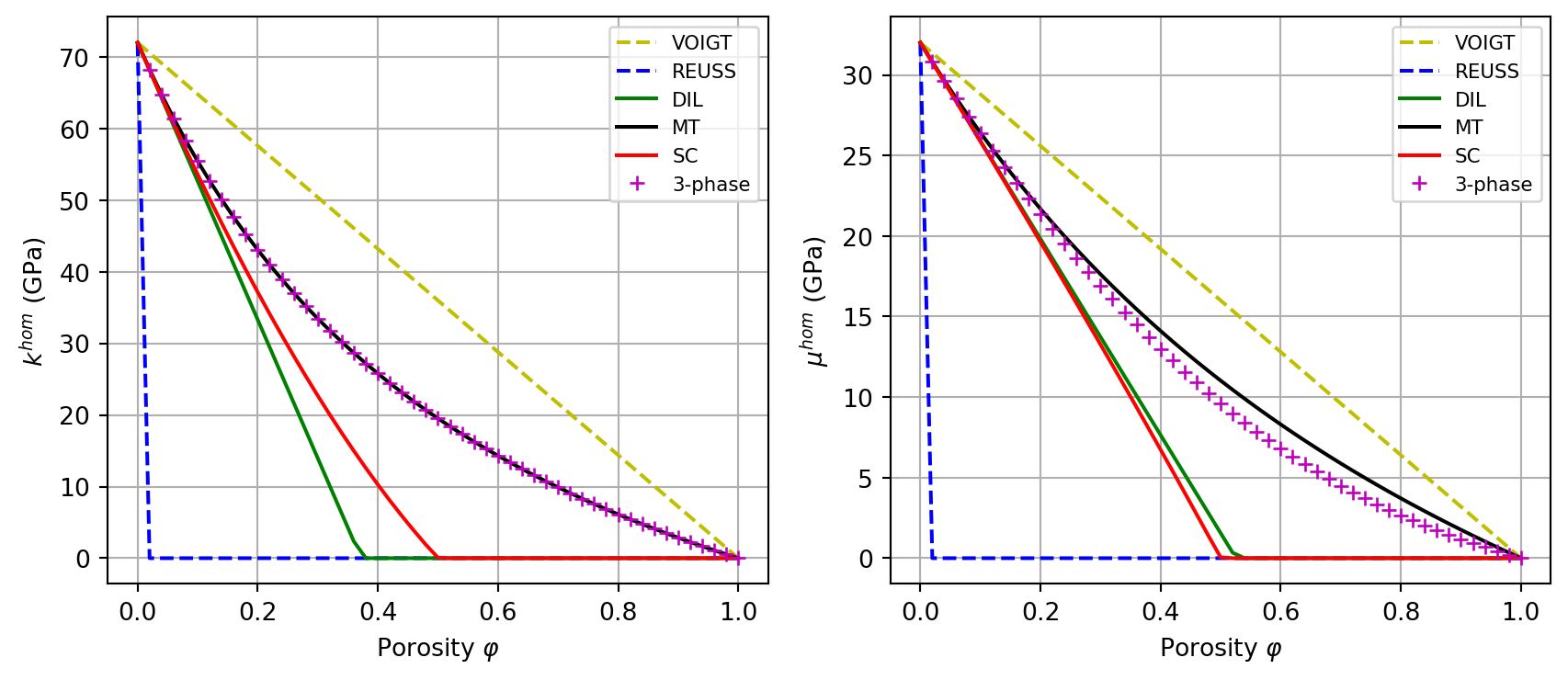

Exercise 2: Multiscale hierarchical structure

Exercise

A 3-phase model is built with a microporous solid: the solid shell of the 2-layer sphere is itself a porous material homogenized at a lower scale.

Consider the following global volume fractions:

solid mineral: $f_s = 0.70$
macropores: $f_M = 0.20$
micropores: $f_m = 0.10$

The solid mineral has the same properties as in Exercise 1 ($k_s=72$ GPa, $\mu_s=32$ GPa).

The microporous solid is obtained at the lower scale by homogenizing a porous solid (Mori-Tanaka scheme, spheroidal pores with aspect ratio $\omega_p=0.2$). Its porosity is $\varphi_\text{low} = f_m / (f_s + f_m)$.

At the upper scale, use a 3-phase SC model: a single sphere_nlayers inclusion with the macropore as inner core (fraction $f_M$) and the microporous solid as outer shell (fraction $1-f_M$).

Solution

fs, fM, fm = 0.7, 0.2, 0.1

# Lower scale: microporous solid via MT (spheroidal pores, omega=0.2)
phi_low = fm / (fs + fm)
Clow = stiff_kmu(*Chom(buildrve(1., 0.2), phi_low, MT))

# Upper scale: 3-phase SC model
rvemacro = rve(matrix="SPN")
rvemacro["SPN"] = sphere_nlayers(radius=1., layer_fractions=[fM, 1 - fM],
                                  fraction=1., prop={"C": [Cp, Clow]})
C = homogenize(prop="C", rve=rvemacro, scheme=SC, verbose=False)

print(f"Lower scale — microporous solid:  k = {Clow.k:.3f} GPa,  mu = {Clow.mu:.3f} GPa")
print(f"Upper scale — homogenized mortar: k = {C.k:.3f} GPa,  mu = {C.mu:.3f} GPa")

Lower scale — microporous solid:  k = 40.447 GPa,  mu = 22.777 GPa
Upper scale — homogenized mortar: k = 25.552 GPa,  mu = 15.117 GPa

Exercise 3: Parameter identification on sandstone

Exercise

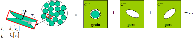
Sandstone can be modelled as a granular assemblage. The grain mineral is isotropic with $k_s = 37$ GPa and $\mu_s = 44$ GPa. A self-consistent scheme is used with:

Grain inclusions: sphere_nlayers with a single layer (sphere of radius 1) and a compliant interface parametrized by normal stiffness $k_n$ and tangential stiffness $k_t$.
Pore inclusions: spheroidal pores with aspect ratio $\omega$.

The following experimental data give $k^{hom}$ and $\mu^{hom}$ (GPa) as a function of porosity:

data_phi = [0.1539, 0.1973, 0.0746, 0.0550, 0.0973, 0.1769, 0.2235]
data_k   = [20.925, 16.748, 28.199, 33.084, 27.536, 20.842, 16.443]
data_mu  = [22.248, 17.766, 30.905, 35.782, 30.317, 19.894, 15.675]

Build the rve for the granular model and a function Chom_sand(f, omega, kn, kt) returning (khom, muhom). Use tZ4 for pore stiffness and PRIMALDISC interface type.
Plot the initial model without softening ($\omega=1$, $k_n = k_t = +\infty$) against the data.
Use nlopt.LN_NELDERMEAD to minimize the sum of squared relative errors on $k$ and $\mu$ over all data points with respect to $(\omega, k_n, k_t)$.
Plot the optimized model vs. data.

Solution

ks_sand = 37.
mus_sand = 44.
Cs_sand = stiff_kmu(ks_sand, mus_sand)

ver = rve()
ver["GRAIN"] = sphere_nlayers(radii=[1.], prop={"C": [Cs_sand]})
ver["PORE"]  = ellipsoid(shape=spherical, symmetrize=[ISO], prop={"C": tZ4})

def Chom_sand(f, omega, kn, kt):
    ver["GRAIN"].fraction = 1. - f
    ver["GRAIN"].set_interf_prop({"C": [[kn, kt, PRIMALDISC]]})
    ver["PORE"].fraction = f
    ver["PORE"].shape = spheroidal(omega)
    C = homogenize(prop="C", rve=ver, scheme=SC, epsrel=1.e-15, maxnb=100)
    return C.k, C.mu

# ── Initial model (no softening: rigid interfaces, spherical pores) ────────
lphi = np.linspace(0., 0.5, 50)
lk0, lmu0 = [], []
for phi in lphi:
    k, mu = Chom_sand(phi, 1., math.inf, math.inf)
    lk0.append(k); lmu0.append(mu)

fig, (ax1, ax2) = plt.subplots(1, 2, figsize=(9, 4))
ax1.plot(data_phi, data_k, 'bo', label="Data")
ax1.plot(lphi, lk0, 'k-', label="No softening")
ax1.set_xlabel(r"$\varphi$"); ax1.set_ylabel(r"$k^{hom}$ (GPa)")
ax1.legend(); ax1.grid(True)
ax2.plot(data_phi, data_mu, 'bo', label="Data")
ax2.plot(lphi, lmu0, 'k-', label="No softening")
ax2.set_xlabel(r"$\varphi$"); ax2.set_ylabel(r"$\mu^{hom}$ (GPa)")
ax2.legend(); ax2.grid(True)
plt.tight_layout()
plt.show()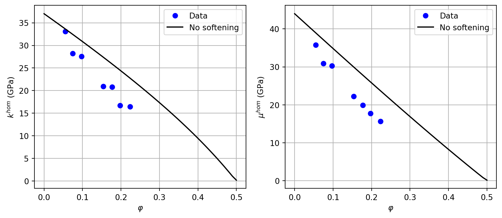

Solution (optimization)

import nlopt

def J(x, grad):
    omega, kn, kt = x[0], x[1], x[2]
    res = 0.
    for i in range(len(data_phi)):
        khom, muhom = Chom_sand(data_phi[i], omega, kn, kt)
        res += (1. - khom / data_k[i])**2 + (1. - muhom / data_mu[i])**2
    return res

opt = nlopt.opt(nlopt.LN_NELDERMEAD, 3)
opt.set_lower_bounds([0.1, 0., 0.])
opt.set_upper_bounds([1., math.inf, math.inf])
opt.set_min_objective(J)
opt.set_xtol_rel(1e-10)
opt.set_maxeval(10000)
opt.set_maxtime(1000)
x_opt = opt.optimize([0.5, 1.e3, 1.e3])

print(f"Optimal pore aspect ratio:  omega = {x_opt[0]:.4f}")
print(f"Optimal interface stiffness: kn = {x_opt[1]:.1f} GPa/m,  kt = {x_opt[2]:.1f} GPa/m")
print(f"Residual J = {opt.last_optimum_value():.6f}")

# ── Comparison plot ────────────────────────────────────────────────────────
lk_opt, lmu_opt = [], []
for phi in lphi:
    k, mu = Chom_sand(phi, *x_opt.tolist())
    lk_opt.append(k); lmu_opt.append(mu)

fig, (ax1, ax2) = plt.subplots(1, 2, figsize=(9, 4))
ax1.plot(data_phi, data_k, 'bo', label="Data")
ax1.plot(lphi, lk0,    'k-', label="No softening")
ax1.plot(lphi, lk_opt, 'g-', label="Optimized")
ax1.set_xlabel(r"$\varphi$"); ax1.set_ylabel(r"$k^{hom}$ (GPa)")
ax1.legend(); ax1.grid(True)
ax2.plot(data_phi, data_mu, 'bo', label="Data")
ax2.plot(lphi, lmu0,    'k-', label="No softening")
ax2.plot(lphi, lmu_opt, 'g-', label="Optimized")
ax2.set_xlabel(r"$\varphi$"); ax2.set_ylabel(r"$\mu^{hom}$ (GPa)")
ax2.legend(); ax2.grid(True)
plt.tight_layout()
plt.show()

Optimal pore aspect ratio:  omega = 0.2139
Optimal interface stiffness: kn = 3576732812105654.0 GPa/m,  kt = 684.8 GPa/m
Residual J = 0.023753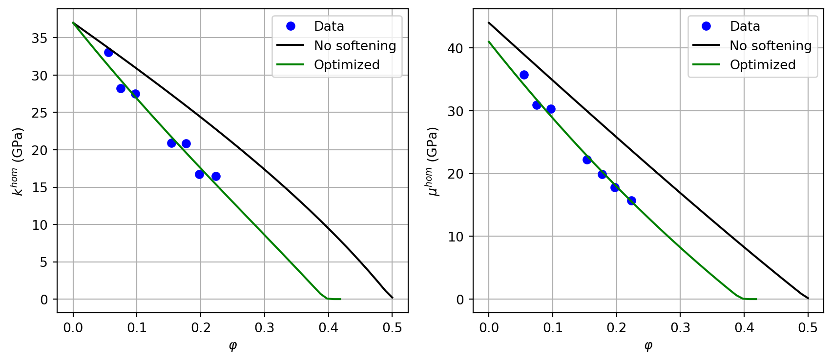

Exercise 4: User-defined inclusion for porous media

Exercise

The user_inclusion class (see Chapter 10) allows supplying the concentration tensors analytically inside build_all(). The goal of this exercise is to re-implement the porous-medium homogenization of Exercise 1 using user_inclusion instead of ellipsoid, and to verify the consistency of the two approaches.

The solid mineral and pore properties are identical to Exercise 1 ($k_s=72$ GPa, $\mu_s=32$ GPa; $k_p=\mu_p=10^{-6}$).

Implement a class MyIncl(user_inclusion) whose build_all() computes the concentration tensors analytically using the Hill polarization tensor for a sphere in an isotropic matrix (see 10.2): \[\uuuu{P} = \frac{1}{3k_0+4\mu_0}\left(\mathbb{J}+\frac{3(k_0+2\mu_0)}{5\mu_0}\,\mathbb{K}\right)\]
Build an rve named ver_usr with solid and pore phases as MyIncl inclusions. Write a function Chom_usr(phi, sch) returning (khom, muhom).
Check that Chom_usr and Chom (from Exercise 1) agree to machine precision for MT and SC at $\varphi=0.3$.
Plot $k^{hom}(\varphi)$ and $\mu^{hom}(\varphi)$ for schemes MT, SC, DIFF, and MAX, comparing the user_inclusion curves (solid lines) with the ellipsoid-based curves from Exercise 1 (dashed lines), and add the 3-phase model from Exercise 1 for reference.

Solution

import math

Cs_u = stiff_kmu(72., 32.)
Cp_u = stiff_kmu(1.e-6, 1.e-6)

class MyIncl(user_inclusion):
    def __init__(self, prop, fraction=0., symmetrize=[]):
        super().__init__(fraction, symmetrize)
        for key, val in prop.items():
            user_inclusion.set_prop(self, key, val)

    def build_all(self):
        C0      = self.ref.array
        S0      = np.linalg.inv(C0)
        k0, mu0 = self.ref.kmu
        Ci = self.prop(self.refname).array
        P  = 1. / (3*k0 + 4*mu0) * (J4 + 3.*(k0 + 2*mu0) / (5*mu0) * K4)
        eE = np.linalg.inv(Id4 + P.dot(Ci - C0))
        eS = eE.dot(S0)
        sE = Ci.dot(eE)
        sS = Ci.dot(eS)
        return {"eE": eE, "eS": eS, "sE": sE, "sS": sS}

ver_usr = rve(matrix="SOLID")
ver_usr["SOLID"] = MyIncl(prop={"C": Cs_u})
ver_usr["PORE"]  = MyIncl(prop={"C": Cp_u})

def Chom_usr(phi, sch):
    ver_usr["PORE"].fraction = phi
    C = homogenize(prop="C", rve=ver_usr, scheme=sch, verbose=False)
    return max(C.k, 0.), max(C.mu, 0.)

# Consistency check vs ellipsoid approach (Exercise 1)
myrve_check = buildrve(1., 1.)
phi_test = 0.3
for sch in [MT, SC]:
    ku, muu = Chom_usr(phi_test, sch)
    ke, mue = Chom(myrve_check, phi_test, sch)
    print(f"{str(sch):4s}  user: k={ku:.6f}  mu={muu:.6f}  |  "
          f"ellipsoid: k={ke:.6f}  mu={mue:.6f}  |  "
          f"err_k={abs(ku-ke):.1e}  err_mu={abs(muu-mue):.1e}")

MT    user: k=33.460582  mu=17.626742  |  ellipsoid: k=33.460582  mu=17.626742  |  err_k=0.0e+00  err_mu=0.0e+00
SC    user: k=22.689245  mu=13.264364  |  ellipsoid: k=22.689235  mu=13.264360  |  err_k=9.9e-06  err_mu=4.5e-06

Solution (plot)

lphi_u = np.linspace(0., 1., 51)
myrve_sph_u = buildrve(1., 1.)

fig, (ax1, ax2) = plt.subplots(1, 2, figsize=(9, 4))

for sch, color in zip([MT, SC, DIFF, MAX], ['k', 'r', 'y', 'm']):
    lk_usr, lmu_usr = [], []
    lk_ell, lmu_ell = [], []
    for phi in lphi_u:
        ku, muu = Chom_usr(phi, sch)
        ke, mue = Chom(myrve_sph_u, phi, sch)
        lk_usr.append(ku); lmu_usr.append(muu)
        lk_ell.append(ke); lmu_ell.append(mue)
    ax1.plot(lphi_u, lk_usr,  color=color, ls='-',  label=f"{str(sch)} user")
    ax1.plot(lphi_u, lk_ell,  color=color, ls='--', label=f"{str(sch)} ell")
    ax2.plot(lphi_u, lmu_usr, color=color, ls='-')
    ax2.plot(lphi_u, lmu_ell, color=color, ls='--')

# 3-phase model from Exercise 1
lk3, lmu3 = [], []
for phi in lphi_u:
    k, mu = Chom3ph(phi)
    lk3.append(k); lmu3.append(mu)
ax1.plot(lphi_u, lk3,  'b+', label="3-phase")
ax2.plot(lphi_u, lmu3, 'b+')

for ax, ylabel in [(ax1, r"$k^{hom}$ (GPa)"), (ax2, r"$\mu^{hom}$ (GPa)")]:
    ax.set_xlabel(r"Porosity $\varphi$")
    ax.set_ylabel(ylabel)
    ax.grid(True)
ax1.legend(fontsize=7, ncol=2)
plt.tight_layout()
plt.show()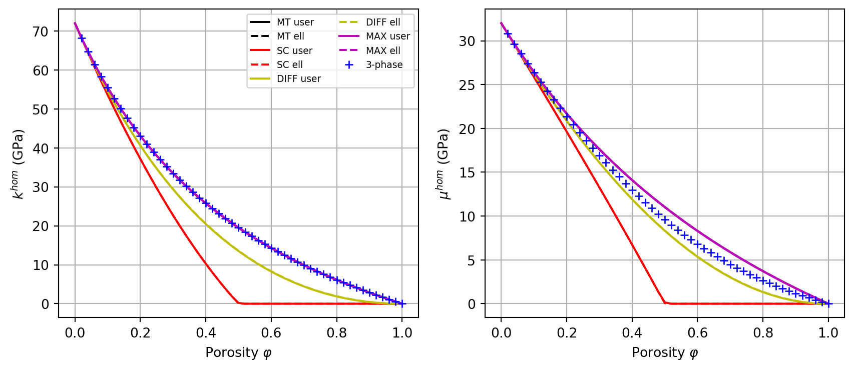

$\,$