import numpy as np
from echoes import *
import math
import matplotlib.pyplot as plt
from scipy.optimize import fsolve

np.set_printoptions(precision=8, suppress=True)19 Nonlinear homogenization and failure criteria
Macroscopic strength domain
Theoretical background
For a porous medium with a solid phase obeying a von Mises criterion with yield stress \(\sigma_0\), the local criterion reads \(\sigma_d \leq \sigma_0\) where \(\sigma_d = \sqrt{\uu{\sigma}':\uu{\sigma}'}\) is the local deviatoric stress norm.
Using the second-order strain moments (see Section 18.1) and the Kreher–Suquet variational result (Kreher, 1990; Suquet, 1997), the macroscopic strength criterion can be expressed in closed form. For isotropic microstructures (using the derivative w.r.t. \(\mu_s\) only), the macroscopic criterion in terms of the mean stress \(\Sigma_m = \tfrac{1}{3}\mathrm{tr}(\uu{\Sigma})\) and deviatoric stress \(\Sigma_d = \sqrt{\uu{\Sigma}':\uu{\Sigma}'}\) is an ellipse:
\[ \frac{\Sigma_m^2}{a^2} + \frac{\Sigma_d^2}{b^2} \leq 1 \tag{19.1}\]
whose semi-axes involve the derivatives of \(k^{hom}\) and \(\mu^{hom}\) with respect to \(\mu_s\):
\[ a = \sigma_0\sqrt{\frac{f_s}{2\,A}}, \quad b = \sigma_0\sqrt{\frac{f_s}{B}} \tag{19.2}\]
with
\[ A = \left(\frac{\mu_s}{k^{hom}}\right)^2\frac{\partial k^{hom}}{\partial \mu_s}, \quad B = \left(\frac{\mu_s}{\mu^{hom}}\right)^2\frac{\partial \mu^{hom}}{\partial \mu_s} \tag{19.3}\]
where the normalized derivatives \(A\) and \(B\) measure the sensitivity of the effective moduli to the solid shear stiffness.
Failure criterion for porous media
Figure — macroscopic failure ellipse (effective modulus derivatives)
def ellipse_radii(ks, mus, f, sch):
    """Compute semi-axes of the macroscopic failure ellipse."""
    myrve = rve(matrix="SOLID")
    myrve["SOLID"] = ellipsoid(shape=spheroidal(0.1), symmetrize=[ISO],
                               prop={"C": stiff_kmu(ks, mus)}, fraction=1 - f)
    myrve["PORE"] = ellipsoid(shape=spheroidal(0.1), symmetrize=[ISO],
                              prop={"C": tZ4}, fraction=f)
    khom, muhom = homogenize(prop="C", rve=myrve, scheme=sch,
                             verbose=False, epsrel=1.e-6, maxnb=300,
                             select_best=True).kmu
    dC = homogenize_derivative(prop="C", rve=myrve, scheme=sch,
                               phase="SOLID", index=1, sym=ISO)
    dCp = dC.paramsym(ISO)
    dkhomdmus = dCp[0] * 2. / 3.
    dmuhomdmus = dCp[1]
    A = (mus / khom)**2 * dkhomdmus
    B = (mus / muhom)**2 * dmuhomdmus
    return math.sqrt((1 - f) / 2. / A), math.sqrt((1 - f) / B)

ks, mus = 1.e6, 1.
ltheta = np.linspace(0., math.pi, 100)
f = 0.15

fig, ax = plt.subplots(figsize=(8, 6))
for sch in [MT, DILD, SC, ASC, PCW, MAX]:
    a, b = ellipse_radii(ks, mus, f, sch)
    ax.plot([a * math.cos(t) for t in ltheta],
            [b * math.sin(t) for t in ltheta],
            label=f"{sch}, φ={f}")

ax.set_aspect('equal')
ax.axhline(color='k'); ax.axvline(color='k')
ax.set_xlabel(r'$\Sigma_m/\sigma_0$')
ax.set_ylabel(r'$\Sigma_d/\sigma_0$')
ax.grid(True); ax.legend(loc='best')
plt.tight_layout()
plt.show()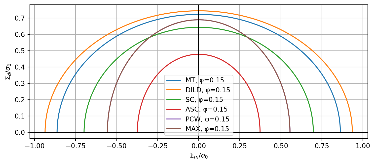
Elastoplastic response of porous media
Modified secant method
The modified secant method (Suquet, 1997) replaces each nonlinear phase by a linear elastic phase with a secant modulus \(\mu^{sec}_r\) chosen so that the second-order strain moment in the linearized composite matches the local yield condition. For a von Mises matrix in phase \(r\) with yield stress \(\sigma_0\):
\[ \mu^{sec}_r = \begin{cases} \mu_s & \text{if } \bar{\varepsilon}_r \leq \varepsilon_0 \\[4pt] \dfrac{\sigma_0}{2\,\bar{\varepsilon}_r} & \text{otherwise} \end{cases} \quad\text{with}\quad \varepsilon_0 = \dfrac{\sigma_0}{2\mu_s} \tag{19.4}\]
where the equivalent strain \(\bar{\varepsilon}_r\) in layer \(r\) is obtained from the second-order moment (see 18.2):
\[ \bar{\varepsilon}_r^2 = \frac{1}{f_r}\left(\frac{1}{2}\frac{\partial k^{hom}}{\partial \mu_r}\,E_v^2 + \frac{\partial \mu^{hom}}{\partial \mu_r}\,E_d^2\right) \tag{19.5}\]
with \(E_v = \mathrm{tr}(\uu{E})\) the volumetric macro-strain and \(E_d^2 = \uu{E}':\uu{E}'\) the deviatoric macro-strain squared. The nonlinear problem is solved by a fixed-point iteration: the matrix is discretized into \(n\) concentric layers (via sphere_nlayers), each carrying a different secant modulus, and the self-consistent scheme is applied until convergence.
Figure — elastoplastic response via modified secant method
def build_rve_ep(n, ks, mus, sigma0, f, tabed):
    eps0 = sigma0 / (2. * mus)
    myrve = rve(matrix="SOLID", prop={"C": tId4})
    tabmu = [mus if abs(tabed[i]) <= eps0
             else sigma0 / (2. * abs(tabed[i])) for i in range(n)]
    myrve["SOLID"] = sphere_nlayers(
        radius=1., fraction=1.,
        layer_fractions=[f] + [(1. - f) / n for _ in range(n)],
        prop={"C": [tZ4] + [stiff_kmu(ks, tabmu[i]) for i in range(n)]})
    return myrve

def Sigma_ep(vE, n, ks, mus, sigma0, f):
    tE = invKM(vE)
    Ev = np.trace(tE); Ev2 = Ev**2
    tEd = tE - (Ev / 3.) * np.eye(3); Ed2 = np.sum(tEd * tEd)

    def buildsys(x):
        sys = []
        myrve = build_rve_ep(n, ks, mus, sigma0, f, x)
        homogenize(prop="C", rve=myrve, scheme=SC,
                   verbose=False, epsrel=1.e-6, maxnb=300)
        for i in range(n):
            dC = homogenize_derivative(prop="C", rve=myrve, scheme=SC,
                                        phase="SOLID", layer=i + 1,
                                        index=1, sym=ISO, verbose=False)
            dCp = dC.paramsym(ISO)
            dkhomdmus = dCp[0] * 2. / 3.
            dmuhomdmus = dCp[1]
            fi = myrve["SOLID"].layer_fraction(i + 1)
            sys.append(math.sqrt((0.5 * dkhomdmus * Ev2
                                  + dmuhomdmus * Ed2) / fi) - x[i])
        return sys

    x0 = (100. * sigma0 / mus * np.ones(n)).tolist()
    xsol = fsolve(buildsys, x0)
    myrve = build_rve_ep(n, ks, mus, sigma0, f, xsol)
    Chom = homogenize(prop="C", rve=myrve, scheme=SC,
                      verbose=False, epsrel=1.e-6, maxnb=300)
    return Chom.array.dot(vE)

# Triaxial loading: isotropic compression E = (Ev/3) * Id
tabE = np.linspace(0., 4.e-3, 100)
vE0 = KM(1. / 3. * np.eye(3))
ks, mus, sigma0, f = 2.e3, 1.e3, 1., 0.1

plt.figure(figsize=(7, 4.5))
for n in [1, 2, 5, 10]:
    tabS = []
    for ee in tabE:
        S = Sigma_ep(ee * vE0, n, ks, mus, sigma0, f)
        tabS.append(np.sum(S[0:3]) / 3.)
    plt.plot(tabE, tabS, label=f"n={n}")

plt.xlabel(r'$E_v/3$'); plt.ylabel(r'$\Sigma_m$')
plt.grid(True); plt.legend()
plt.tight_layout()
plt.show()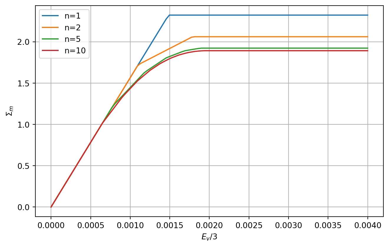
\(\,\)