import numpy as np
from echoes import *
import math
import matplotlib.pyplot as plt
from cmath import phase

np.set_printoptions(precision=8, suppress=True)16 Complex-valued homogenization
Complex-valued tensors
Tensors in Echoes accept complex scalars:
C = stiff_kmu(20 + 2j, 10 + 1j)
print(C)
Order 4 ISO tensor | Param(size=2)=[ (60,6) (20,2) ] | Angles(size=0)=[ ]
[ (33.3333,3.33333) (13.3333,1.33333) (13.3333,1.33333) (0,0) (0,0) (0,0)
(13.3333,1.33333) (33.3333,3.33333) (13.3333,1.33333) (0,0) (0,0) (0,0)
(13.3333,1.33333) (13.3333,1.33333) (33.3333,3.33333) (0,0) (0,0) (0,0)
(0,0) (0,0) (0,0) (20,2) (0,0) (0,0)
(0,0) (0,0) (0,0) (0,0) (20,2) (0,0)
(0,0) (0,0) (0,0) (0,0) (0,0) (20,2) ]
When problems require complex values even though initial moduli are real, multiply by a complex unit:
un = 1 + 0j
C = stiff_kmu(5., 3.)
print((un * C).kmu)
((5+0j), (3+0j))Complex Echoes objects
Objects for complex-valued calculations differ from their real counterparts by an additional suffix c:
| Real | Complex |
|---|---|
ellipsoid |
ellipsoidc |
sphere_nlayers |
sphere_nlayersc |
rve |
rvec |
un = 1 + 0j
Cs = un * stiff_kmu(72., 32.)
Cp = un * stiff_kmu(1.e-6, 1.e-6)

rve3ph = rvec(matrix="SPN")
rve3ph["SPN"] = sphere_nlayersc(radii=[0.5, 1.], fraction=1.,
                                prop={"C": [Cp, Cs]})
C = homogenize(prop="C", rve=rve3ph, scheme=SC, verbose=True)
print(C)
print(C.kmu)
Order 4 ISO tensor | Param(size=2)=[ (156.077,0) (50.1115,0) ] | Angles(size=0)=[ ]
[ (85.4335,0) (35.322,0) (35.322,0) (0,0) (0,0) (0,0)
(35.322,0) (85.4335,0) (35.322,0) (0,0) (0,0) (0,0)
(35.322,0) (35.322,0) (85.4335,0) (0,0) (0,0) (0,0)
(0,0) (0,0) (0,0) (50.1115,0) (0,0) (0,0)
(0,0) (0,0) (0,0) (0,0) (50.1115,0) (0,0)
(0,0) (0,0) (0,0) (0,0) (0,0) (50.1115,0) ]
((52.02580706730485+0j), (25.055768065145173+0j))Application: complex modulus of a mastic
A mastic is composed of a bituminous matrix and fine elastic aggregates.
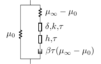
The bitumen obeys a linear viscoelastic behavior with constant bulk modulus \(k^b=2500\) MPa and complex shear modulus \(\mu^*(i\omega)\) of the 2S2P1D type:
\[ \mu^*(p)=\mu_0+\frac{\mu_\infty-\mu_0}{1+(p\,\tau)^{-h}+\delta\,(p\,\tau)^{-k}+(p\,\tau\,\beta)^{-1}} \tag{16.1}\]
The aggregates are elastic with \(E=95000\) MPa, \(\nu=0.17\). The volume fraction of fines is 30%.
Figure — complex modulus of mastic: frequency diagrams (2S2P1D + MT)
class Mod2S2P1D(dict):
    def __init__(self, Mo, Moo, delta, tau, k, h, beta):
        super().__init__({"Mo": Mo, "Moo": Moo, "delta": delta,
                         "tau": tau, "k": k, "h": h, "beta": beta})
    def __call__(self, p):
        return self["Mo"] + (self["Moo"] - self["Mo"]) / \
            (1. + self["delta"] * (p * self["tau"])**(-self["k"])
             + (p * self["tau"])**(-self["h"])
             + 1. / (p * self["beta"] * self["tau"]))

mub = Mod2S2P1D(0., 900., 3., 3.e-5, 0.22, 0.6, 500.)

myrve = rvec(matrix="BITUMEN")
myrve["BITUMEN"] = ellipsoidc(shape=spherical, fraction=0.7)
myrve["FINES"] = ellipsoidc(shape=spherical, fraction=0.3,
    prop={"C": (1 + 0j) * stiff_Enu(95000., 0.17)})

def Chom_freq(p):
    myrve["BITUMEN"].set_prop("C", stiff_kmu(2500 + 0j, mub(p)))
    return homogenize(prop="C", rve=myrve, scheme=MT)

lw = np.logspace(-5, 16, 100)
lC = [Chom_freq(1j * w) for w in lw]
labsE = [abs(C.E) for C in lC]
lphi = [180 / math.pi * phase(C.E) for C in lC]
lE1 = [C.E.real for C in lC]
lE2 = [C.E.imag for C in lC]

fig, axes = plt.subplots(2, 2, figsize=(9, 7.5))

axes[0, 0].loglog(lw, labsE, 'r-')
axes[0, 0].grid(True, which='both')
axes[0, 0].set_xlabel(r"$\omega$"); axes[0, 0].set_ylabel(r"$|E^*|$")

axes[0, 1].semilogx(lw, lphi, 'r-')
axes[0, 1].grid(True, which='both')
axes[0, 1].set_xlabel(r"$\omega$"); axes[0, 1].set_ylabel(r"$\varphi_E$ (°)")

axes[1, 0].plot(lE1, lE2, 'r-')
axes[1, 0].grid(True)
axes[1, 0].set_xlabel(r"$E_1$"); axes[1, 0].set_ylabel(r"$E_2$")
axes[1, 0].set_title("Cole-Cole diagram")

axes[1, 1].semilogy(lphi, labsE, 'r-')
axes[1, 1].grid(True, which='both')
axes[1, 1].set_xlabel(r"$\varphi_E$ (°)"); axes[1, 1].set_ylabel(r"$|E^*|$")
axes[1, 1].set_title("Black diagram")

plt.tight_layout()
plt.show()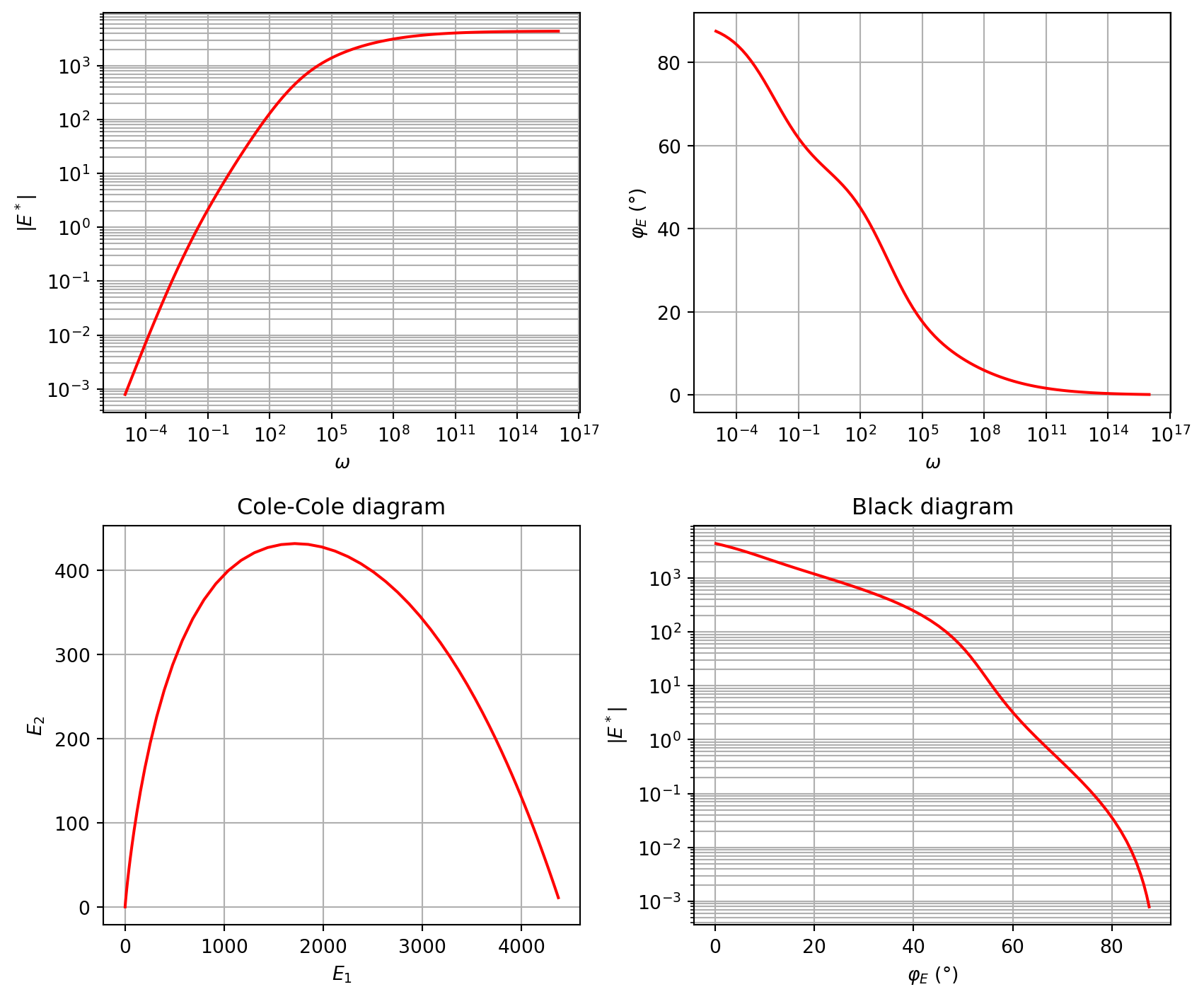
\(\,\)