import numpy as np
from echoes import *
import matplotlib.pyplot as plt

np.set_printoptions(precision=5, suppress=True)22 Cement paste: chloride diffusivity and elasticity
Volume fractions: Powers’ hydration model
The volume fractions of the main phases are derived from Powers’ hydration model as functions of \(w/c\) and \(\alpha\) (Achour et al., 2020):
\[ f_a = \frac{1-\alpha}{1+\rho_a\,w/c}, \quad f_h = \frac{\kappa_h\,\alpha}{1+\rho_a\,w/c}, \quad f_{cp} = 1 - f_a - f_h \]
with \(\rho_a=3.13\) (clinker density), \(\kappa_h=2.13\) (hydrate expansion factor). When excess water is available, hydration stops when the pore space is filled:
\[ \alpha_{\max} = \min\!\left(1,\;\frac{\rho_a\,w/c}{\kappa_h-1}\right) \]
The Tennis–Jennings correlation (Tennis and Jennings, 2000) provides the mass ratio \(M_r\) of low-density (LD) to total C-S-H:
\[ M_r = \min\!\Bigl(1,\;0.538 + \alpha(3.017\,w/c - 1.347)\Bigr) \]
This splits the hydration products into an inner layer (HD-C-S-H, \(\phi_{HD}=0.24\)) and an outer layer (LD-C-S-H, \(\phi_{LD}=0.37\)), with a fraction \(\eta=20\%\) of crystalline hydrates (portlandite) in each.
Volume fractions — Powers and Tennis-Jennings hydration models
# Powers' hydration model constants
rho_a   = 3.13   # clinker-to-water density ratio
kappa_h = 2.13   # volume of hydrates / unit volume of clinker
eta     = 0.20   # crystalline hydrate fraction in hydration products
phi_HD  = 0.24   # HD-CSH gel porosity
phi_LD  = 0.37   # LD-CSH gel porosity
phi_od0 = 0.63   # initial SCP fraction in outer domain (Ma 2014 fit)

def alphamax(wc):
    return min(1., wc * rho_a / (kappa_h - 1.))

def fa(wc, alpha):   return (1. - alpha) / (1. + rho_a * wc)
def fh(wc, alpha):   return kappa_h * alpha / (1. + rho_a * wc)
def fcp(wc, alpha):  return max(0., 1. - fa(wc, alpha) - fh(wc, alpha))

# Tennis-Jennings LD/HD mass ratio and LD volume fraction
def mLD(wc, alpha):
    return min(1., 0.538 + alpha * (3.017 * wc - 1.347))

def muLD(wc, alpha):
    mr = mLD(wc, alpha)
    return mr * (1. - phi_HD) / (1. - phi_LD + mr * (phi_LD - phi_HD))

# Inner (HD-based) and outer (LD-based) hydration products
def fihp(wc, alpha): return (1. - muLD(wc, alpha)) * fh(wc, alpha)
def fohp(wc, alpha): return muLD(wc, alpha) * fh(wc, alpha)

# SCP (small, 3-100 nm) and LCP (large, >100 nm) capillary pore fractions
def psif(wc, alpha):
    denom = 1. - fa(wc, alpha) - fihp(wc, alpha)
    return 0. if denom < 1.e-12 else fohp(wc, alpha) / denom

def fscp(wc, alpha):
    phi = phi_od0 * (1. - psif(wc, alpha))
    return fohp(wc, alpha) * phi / max(1. - phi, 1.e-12)

def flcp(wc, alpha):
    return max(0., fcp(wc, alpha) - fscp(wc, alpha))
Engineering model
The engineering model (Achour et al., 2020; Pichler and Hellmich, 2011) involves two homogenization steps:
- Level I — hydrate foam (self-consistent): an aging disordered assemblage of hydration products and capillary pores. The hydrates are modeled as oblate spheroids (\(\omega_h = 0.013\)) so that the solid phase percolates at the experimentally observed setting degree; the capillary pores are prolate (\(\omega_{cp} = 6\)) to maintain a connected pore network throughout hydration.
- Level II — cement paste (Mori-Tanaka): spherical anhydrous clinker inclusions embedded in the hydrate foam matrix.
The same phase properties serve both the mechanical and the diffusion problems. All diffusivities are normalized by the bulk-water value \(D_\text{bulk}=1\).
Function engineering_model() — two-scale homogenization (SC + MT)
# Material properties — engineering model
C_anhyd = stiff_Enu(135., 0.3)    # anhydrous clinker
C_hyd   = stiff_Enu(25.3, 0.29)   # hydration products (calibrated, see text)
D_hyd   = 5.04e-4 * tId2          # hydrate diffusivity (calibrated to Yu 1991)
D_cap   = tId2                    # capillary pore: D_bulk = 1

# Aspect ratios (calibrated from setting experiments)
omega_h  = 0.013   # oblate hydrates
omega_cp = 6.      # prolate capillary pores

def engineering_model(wc, alpha=-1.):
    if alpha < 0.: alpha = alphamax(wc)
    _fa  = fa(wc, alpha)
    _fh  = fh(wc, alpha)
    _fcp = fcp(wc, alpha)
    ft   = _fh + _fcp            # foam total fraction (= 1 - fa)
    if ft < 1.e-10: return None, None

    # Level I: hydrate foam (SC)
    ver_foam = rve()
    ver_foam["HYD"] = ellipsoid(shape=spheroidal(omega_h),  symmetrize=[ISO],
                                fraction=_fh  / ft, prop={"C": C_hyd, "D": D_hyd})
    ver_foam["CAP"] = ellipsoid(shape=spheroidal(omega_cp), symmetrize=[ISO],
                                fraction=_fcp / ft, prop={"C": tZ4,   "D": D_cap})
    try:
        C_foam = homogenize(prop="C", rve=ver_foam, scheme=SC,
                            verbose=False, epsrel=1.e-10, maxnb=300)
        D_foam = homogenize(prop="D", rve=ver_foam, scheme=SC,
                            verbose=False, epsrel=1.e-10, maxnb=300)
        # Skip if foam has not yet percolated (zero stiffness → singular MT matrix)
        if C_foam.k < 1.e-6:
            return 0., np.trace(D_foam.array) / 3.

        # Level II: cement paste (MT — clinker inclusions in foam matrix)
        ver_paste = rve(matrix="FOAM")
        ver_paste["FOAM"]   = ellipsoid(shape=spherical, fraction=1. - _fa,
                                        prop={"C": C_foam, "D": D_foam})
        ver_paste["CLINKER"]= ellipsoid(shape=spherical, fraction=_fa,
                                        prop={"C": C_anhyd, "D": tZ2})
        C_cp = homogenize(prop="C", rve=ver_paste, scheme=MT, verbose=False)
        D_cp = homogenize(prop="D", rve=ver_paste, scheme=MT, verbose=False)
        return C_cp.E, np.trace(D_cp.array) / 3.
    except Exception:
        return None, None
Figure — effective modulus and diffusivity (engineering model)
wc_list = [0.30, 0.40, 0.50, 0.60]
n_alpha = 40

fig, (ax1, ax2) = plt.subplots(1, 2, figsize=(9, 4))

for wc in wc_list:
    la = np.linspace(0.02, alphamax(wc), n_alpha)
    lE, lD = [], []
    for alpha in la:
        E, D = engineering_model(wc, alpha)
        lE.append(E if E is not None else np.nan)
        lD.append(D if D is not None else np.nan)
    ax1.plot(la, lE,   label=f"w/c={wc}")
    ax2.semilogy(la, lD, label=f"w/c={wc}")

ax1.set_xlabel(r"$\alpha$"); ax1.set_ylabel(r"$E^{hom}$ (GPa)")
ax1.set_xlim(0., 1.); ax1.set_ylim(bottom=0.)
ax1.set_title("Young's modulus"); ax1.grid(True); ax1.legend()

ax2.set_xlabel(r"$\alpha$"); ax2.set_ylabel(r"$D^{hom}/D_{bulk}$")
ax2.set_xlim(0., 1.)
ax2.set_title("Chloride diffusivity"); ax2.grid(True, which="both"); ax2.legend()

plt.suptitle("Engineering model", y=1.01)
plt.tight_layout()
plt.show()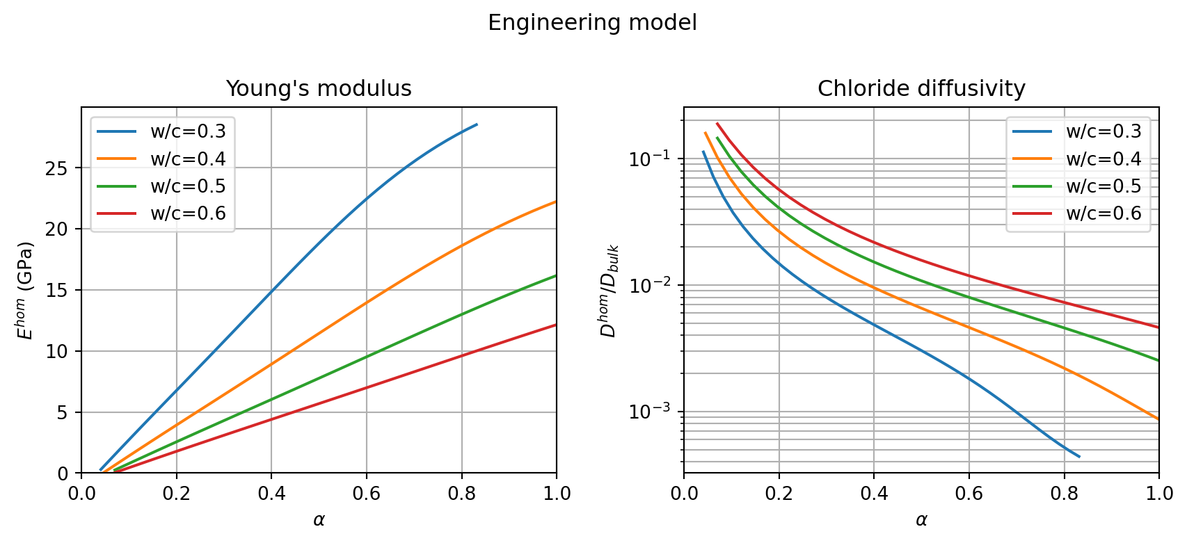
Detailed model
The detailed three-scale model explicitly tracks C-S-H gel microstructure at the nanometre scale, the inner/outer hydrate layers at the micrometre scale, and the cement paste assembly at the grain scale.
Level 0: C-S-H gels
Both HD- and LD-C-S-H gels are modeled as a SC assemblage of:
- Oblate solid bricks (\(\omega_s = 0.12\), \(E=63\) GPa, \(\nu=0.27\), \(D=0\)) — based on the 60×30×5 nm dimensions observed for elementary C-S-H particles.
- Prolate gel pores (\(\omega_p = 1/\omega_s \approx 8.3\), \(D_{gel} = 0.025\,D_{bulk}\)) — the elongated shape is required to ensure non-zero diffusivity through both gel types (oblate or spherical pores would yield zero diffusivity at the HD-CSH porosity \(\phi_{HD}=0.24\)).
The gel properties are fixed (independent of \(w/c\) and \(\alpha\)) and pre-computed once.
Function homogenize_csh() — C-S-H gel at nanoscale (SC)
# Level 0: C-S-H gel microstructure
omega_s = 0.12          # solid C-S-H brick (oblate)
omega_p = 1. / omega_s  # gel pore (prolate, ≈ 8.3)
C_brick  = stiff_Enu(63., 0.27)    # solid C-S-H brick
C_crystal= stiff_Enu(42.3, 0.324)  # crystalline hydrate (portlandite)
D_gel    = 0.025 * tId2            # gel pore diffusivity
D_cap    = tId2                    # capillary pore diffusivity = D_bulk

def homogenize_csh(phi):
    """SC estimate of a C-S-H gel foam at gel porosity phi."""
    ver = rve()
    ver["BRICK"] = ellipsoid(shape=spheroidal(omega_s), symmetrize=[ISO],
                             fraction=1. - phi, prop={"C": C_brick, "D": tZ2})
    ver["PORE"]  = ellipsoid(shape=spheroidal(omega_p), symmetrize=[ISO],
                             fraction=phi,     prop={"C": tZ4,    "D": D_gel})
    C_g = homogenize(prop="C", rve=ver, scheme=SC, verbose=False,
                     epsrel=1.e-10, maxnb=300)
    D_g = homogenize(prop="D", rve=ver, scheme=SC, verbose=False,
                     epsrel=1.e-10, maxnb=300)
    return C_g, D_g

# Pre-compute HD and LD C-S-H gel properties (fixed)
C_HD, D_HD = homogenize_csh(phi_HD)
C_LD, D_LD = homogenize_csh(phi_LD)

print(f"HD-CSH: E = {C_HD.E:.2f} GPa,  D/D_bulk = {np.trace(D_HD.array)/3.:.4e}")
print(f"LD-CSH: E = {C_LD.E:.2f} GPa,  D/D_bulk = {np.trace(D_LD.array)/3.:.4e}")
HD-CSH: E = 31.04 GPa, D/D_bulk = 4.4318e-04
LD-CSH: E = 17.59 GPa, D/D_bulk = 1.5964e-03Level I: inner and outer hydrate layers
Inner layer (HD-C-S-H + nano-crystals, SC, spherical particles):
\[ \text{inner} = \text{SC}\!\left[(1-\eta)\,\text{HD-CSH}_\text{foam} + \eta\,\text{nano-crystals}\right] \]
Outer C-S-H layer (LD-C-S-H + small capillary pores, SC):
\[ \text{outer-CSH} = \text{SC}\!\left[\frac{(1-\eta)f_{ohp}}{f_{scp}+(1-\eta)f_{ohp}}\, \text{LD-CSH}_{\omega_{LD}=0.14} + \frac{f_{scp}}{f_{scp}+(1-\eta)f_{ohp}}\, \text{SCP}_\text{spherical}\right] \]
The oblate LD-C-S-H foam aspect ratio \(\omega_{LD} = 0.14\) controls the setting threshold of the outer layer. Micro-crystals (fraction \(\eta f_{ohp}/(f_{scp}+f_{ohp})\) of the outer domain) are folded into the outer layer by a second SC step.
Functions inner/outer_layer_props() — hydrate layers
omega_LD = 0.14    # oblate LD-CSH foam (calibrated to setting data)

def inner_layer_props(wc, alpha):
    """SC: HD-CSH gel + spherical nano-crystals."""
    eta_inner = eta   # crystal fraction in inner layer
    ver = rve()
    ver["CSH"]     = ellipsoid(shape=spherical, fraction=1. - eta_inner,
                               prop={"C": C_HD, "D": D_HD})
    ver["CRYSTAL"] = ellipsoid(shape=spherical, fraction=eta_inner,
                               prop={"C": C_crystal, "D": tZ2})
    C_in = homogenize(prop="C", rve=ver, scheme=SC, verbose=False,
                      epsrel=1.e-10, maxnb=300)
    D_in = homogenize(prop="D", rve=ver, scheme=SC, verbose=False,
                      epsrel=1.e-10, maxnb=300)
    return C_in, D_in

def outer_layer_props(wc, alpha):
    """SC: LD-CSH gel + SCP → outer CSH; then SC: outer CSH + micro-crystals."""
    _fohp = fohp(wc, alpha)
    _fscp = fscp(wc, alpha)
    f_ldcsh = (1. - eta) * _fohp        # LD-CSH foam volume in outer domain
    f_outer_total = f_ldcsh + _fscp     # LD-CSH + SCP
    if f_outer_total < 1.e-12:
        return C_LD, D_LD

    phi_scp = _fscp / f_outer_total     # SCP fraction within LD-CSH+SCP mix

    # Step 1: SC of oblate LD-CSH foam + spherical SCPs
    ver_csh_scp = rve()
    ver_csh_scp["LDCSH"] = ellipsoid(shape=spheroidal(omega_LD), symmetrize=[ISO],
                                     fraction=1. - phi_scp,
                                     prop={"C": C_LD, "D": D_LD})
    ver_csh_scp["SCP"]   = ellipsoid(shape=spherical, fraction=phi_scp,
                                     prop={"C": tZ4,  "D": D_cap})
    C_csh_scp = homogenize(prop="C", rve=ver_csh_scp, scheme=SC,
                            verbose=False, epsrel=1.e-10, maxnb=300)
    D_csh_scp = homogenize(prop="D", rve=ver_csh_scp, scheme=SC,
                            verbose=False, epsrel=1.e-10, maxnb=300)

    # Step 2: SC of outer CSH layer + spherical micro-crystals
    eta_outer = eta * _fohp / (_fohp + _fscp)  # micro-crystal fraction
    ver_outer = rve()
    ver_outer["CSH"]     = ellipsoid(shape=spherical, fraction=1. - eta_outer,
                                     prop={"C": C_csh_scp, "D": D_csh_scp})
    ver_outer["CRYSTAL"] = ellipsoid(shape=spherical, fraction=eta_outer,
                                     prop={"C": C_crystal, "D": tZ2})
    C_out = homogenize(prop="C", rve=ver_outer, scheme=SC,
                        verbose=False, epsrel=1.e-10, maxnb=300)
    D_out = homogenize(prop="D", rve=ver_outer, scheme=SC,
                        verbose=False, epsrel=1.e-10, maxnb=300)
    return C_out, D_out
Level II: cement paste
At the largest scale, the cement paste is assembled using a generalized self-consistent scheme with two inclusion types:
- a
sphere_nlayerscomposite: anhydrous clinker (core) + inner layer + outer layer, with layer thickness ratios determined by the volume fractions; - spherical large capillary pores (LCPs, \(D = D_{bulk}\)).
The sphere_nlayers constructor with layer_fractions takes the three layer volume fractions (relative to the whole paste) and automatically computes the layer radii.
Function detailed_model() — three-scale detailed model
def detailed_model(wc, alpha=-1.):
    if alpha < 0.: alpha = alphamax(wc)
    try:
        _fa   = fa(wc, alpha)
        _fihp = fihp(wc, alpha)
        _fohp = fohp(wc, alpha)
        _fscp = fscp(wc, alpha)
        _flcp = flcp(wc, alpha)
        f_layers = _fa + _fihp + _fohp + _fscp  # total sphere_nlayers fraction

        # Level I properties
        C_inner, D_inner = inner_layer_props(wc, alpha)
        C_outer, D_outer = outer_layer_props(wc, alpha)

        # Level II: generalized SC — composite sphere + LCPs
        ver_paste = rve()
        ver_paste["LAYERS"] = sphere_nlayers(
            radius=1.,
            layer_fractions=[_fa, _fihp, _fohp + _fscp],
            fraction=f_layers,
            prop={"C": [C_anhyd, C_inner, C_outer],
                  "D": [tZ2,    D_inner, D_outer]})
        ver_paste["LCP"] = ellipsoid(shape=spherical, fraction=_flcp,
                                     prop={"C": tZ4, "D": D_cap})

        C_cp = homogenize(prop="C", rve=ver_paste, scheme=SC,
                          verbose=False, epsrel=1.e-10, maxnb=300)
        D_cp = homogenize(prop="D", rve=ver_paste, scheme=SC,
                          verbose=False, epsrel=1.e-10, maxnb=300)
        return C_cp.E, np.trace(D_cp.array) / 3.
    except Exception:
        return None, None
Figure — effective modulus and diffusivity (detailed model)
fig, (ax1, ax2) = plt.subplots(1, 2, figsize=(9, 4))

for wc in wc_list:
    la = np.linspace(0.02, alphamax(wc), n_alpha)
    lE, lD = [], []
    for alpha in la:
        E, D = detailed_model(wc, alpha)
        lE.append(E if E is not None else np.nan)
        lD.append(D if D is not None else np.nan)
    ax1.plot(la, lE,   label=f"w/c={wc}")
    ax2.semilogy(la, lD, label=f"w/c={wc}")

ax1.set_xlabel(r"$\alpha$"); ax1.set_ylabel(r"$E^{hom}$ (GPa)")
ax1.set_xlim(0., 1.); ax1.set_ylim(bottom=0.)
ax1.set_title("Young's modulus"); ax1.grid(True); ax1.legend()

ax2.set_xlabel(r"$\alpha$"); ax2.set_ylabel(r"$D^{hom}/D_{bulk}$")
ax2.set_xlim(0., 1.)
ax2.set_title("Chloride diffusivity"); ax2.grid(True, which="both"); ax2.legend()

plt.suptitle("Detailed model", y=1.01)
plt.tight_layout()
plt.show()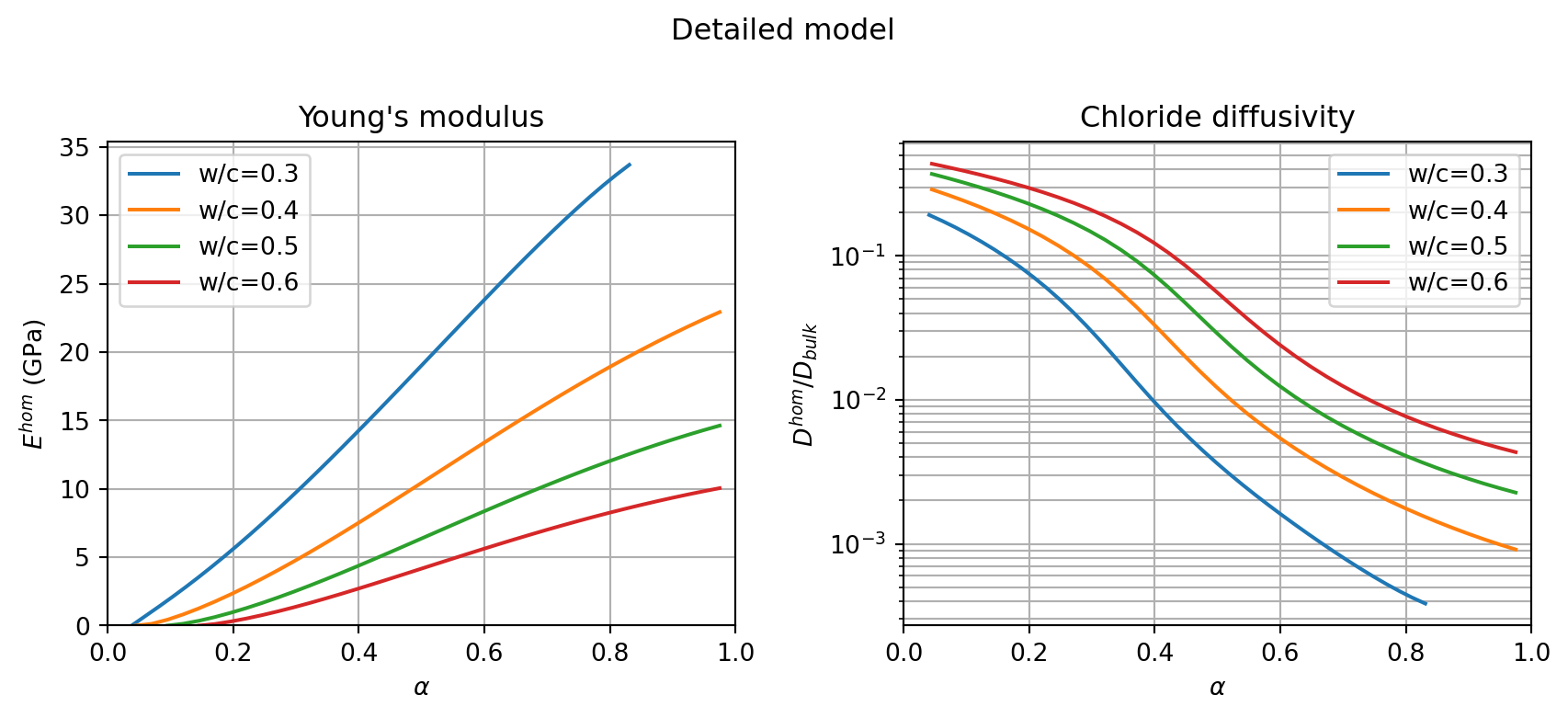
Comparison of both models
The two models predict consistent trends for both elastic moduli and chloride diffusivity throughout hydration. The engineering model is significantly faster but relies on effective hydrate properties calibrated from mature paste data. The detailed model is richer in microstructural content and yields closer agreement with experimental data across the full hydration range and a wider range of \(w/c\) (Achour et al., 2020).
For a given \(w/c\), both models predict:
- a percolation threshold in stiffness around the experimentally observed setting degree (controlled by the calibrated oblate aspect ratios);
- a sharp drop in diffusivity at intermediate to high hydration degrees, as the large capillary pore network becomes disconnected and diffusion is forced through the poorly-diffusive gel pores.
Figure — engineering vs detailed model comparison
wc = 0.4
la = np.linspace(0.02, alphamax(wc), n_alpha)
lE_eng, lD_eng, lE_det, lD_det = [], [], [], []
for alpha in la:
    E1, D1 = engineering_model(wc, alpha)
    E2, D2 = detailed_model(wc, alpha)
    lE_eng.append(E1 if E1 is not None else np.nan)
    lD_eng.append(D1 if D1 is not None else np.nan)
    lE_det.append(E2 if E2 is not None else np.nan)
    lD_det.append(D2 if D2 is not None else np.nan)

fig, (ax1, ax2) = plt.subplots(1, 2, figsize=(9, 4))
ax1.plot(la, lE_eng, 'b--', label="engineering")
ax1.plot(la, lE_det, 'r-',  label="detailed")
ax1.set_xlabel(r"$\alpha$"); ax1.set_ylabel(r"$E^{hom}$ (GPa)")
ax1.set_title(f"Young's modulus — w/c={wc}")
ax1.set_xlim(0., 1.); ax1.set_ylim(bottom=0.)
ax1.grid(True); ax1.legend()

ax2.semilogy(la, lD_eng, 'b--', label="engineering")
ax2.semilogy(la, lD_det, 'r-',  label="detailed")
ax2.set_xlabel(r"$\alpha$"); ax2.set_ylabel(r"$D^{hom}/D_{bulk}$")
ax2.set_title(f"Chloride diffusivity — w/c={wc}")
ax2.set_xlim(0., 1.)
ax2.grid(True, which="both"); ax2.legend()

plt.tight_layout()
plt.show()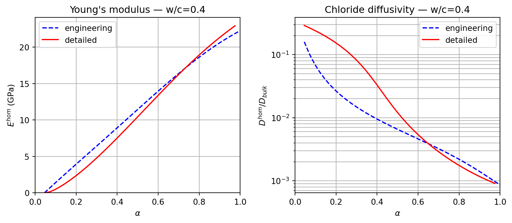
\(\,\)
SC percolation diagrams: role of inclusion shapes
In the SC scheme for a two-phase assemblage of solid spheroids (aspect ratio \(\omega_s\)) and pore spheroids (aspect ratio \(\omega_p\)), the elastic and diffusion percolation thresholds depend strongly on the shape of both phases. These diagrams — established in Achour et al. (2020) — provide the geometrical basis for calibrating the aspect ratios \(\omega_h\) and \(\omega_{cp}\) of the engineering model.
Two percolation thresholds are computed for a two-phase medium with solid (\(\uuuu{C}_s\neq\uuuu{0}\), \(\uu{D}_s=\uu{0}\)) and pore (\(\uuuu{C}_p=\uuuu{0}\), \(\uu{D}_p\neq\uu{0}\)) phases; the threshold fractions depend only on inclusion shapes, not on the actual (non-zero) values of \(\uuuu{C}_s\) and \(\uu{D}_p\):
- Elastic threshold \(\phi_e^{\rm elas}\): the critical pore fraction above which \(\uuuu{C}^{\rm hom}=\uuuu{0}\) (solid skeleton ceases to carry load). Introducing the second Hill polarization tensor \(\uuuu{Q}_p(\nu)=\uuuu{C}(\nu)-\uuuu{C}(\nu):\uuuu{P}(\omega_p,\uuuu{C}(\nu)):\uuuu{C}(\nu)\) (see 5.6), where \(\uuuu{C}(\nu)=\uuuu{C}^{\rm hom}\) denotes the SC homogenised medium normalised to unit Young’s modulus, the SC equation at \(\uuuu{C}^{\rm hom}\to\uuuu{0}^+\) reduces to the coupled system in \((f_s,\nu)\), \(\nu\) being the Poisson’s ratio of the SC medium (not a prescribed solid property):
\[ f_s = \frac{\tr(\uuuu{J}:\uuuu{Q}_p^{-1})}{(1-2\nu)^2\,\tr(\uuuu{J}:\uuuu{P}_s^{-1})+\tr(\uuuu{J}:\uuuu{Q}_p^{-1})}, \qquad f_s\,(1+\nu)^2\,\tr(\uuuu{K}:\uuuu{P}_s^{-1}) = (1-f_s)\,\tr(\uuuu{K}:\uuuu{Q}_p^{-1}) \]
where \(\uuuu{P}_s=\uuuu{P}(\omega_s,\uuuu{C}(\nu))\) is the Hill tensor of the solid and \(\uuuu{Q}_p=\uuuu{C}(\nu)-\uuuu{C}(\nu):\uuuu{P}(\omega_p,\uuuu{C}(\nu)):\uuuu{C}(\nu)\) is the second Hill polarization tensor of the pore; \(\phi_e^{\rm elas}=1-f_s\).
- Diffusion threshold \(\phi_e^{\rm diff}\): the critical porosity above which the pore network is connected (\(\uu{D}^{\rm hom}>\uu{0}\)). It follows analytically from the second-order SC equation at \(\uu{D}^{\rm hom}\to\uu{0}^+\):
\[ \phi_e^{\rm diff} = \frac{\tr\,\uu{Q}_s^{-1}}{\tr\,\uu{P}_p^{-1}+\tr\,\uu{Q}_s^{-1}} \]
where \(\uu{P}_p=\uu{P}(\omega_p,\uu{I})\) and \(\uu{Q}_s=\uu{I}-\uu{P}(\omega_s,\uu{I})\) are respectively the second-order Hill tensor of the pore and the second Hill polarization tensor of the solid in the diffusion reference medium \(\uu{I}\).
from scipy.optimize import bisect
import plotly.graph_objects as go

def felas(omega_s, omega_p):
    """Elastic percolation: returns (f_solid, nu) at C_hom → 0+ (SC two-phase)."""
    ells = spheroidal(omega_s, limit_aspect_ratio=1.e-6)
    ellp = spheroidal(omega_p, limit_aspect_ratio=1.e-6)
    def solf(iPs, iQp, nu):
        tiP = np.trace(J4.dot(iPs))
        tiQ = np.trace(J4.dot(iQp))
        return tiQ / ((1-2*nu)**2 * tiP + tiQ)          # solid fraction at threshold
    def eqnu(nu):
        C = stiff_Enu(1., nu)
        iPs = np.linalg.inv(hill(ells, C))
        iQp = np.linalg.inv(hill_dual(ellp, C))
        f = solf(iPs, iQp, nu)
        tiP = np.trace(K4.dot(iPs))
        tiQ = np.trace(K4.dot(iQp))
        return f * (1+nu)**2 * tiP - (1. - f) * tiQ
    nu    = bisect(eqnu, 0., 0.4)
    C     = stiff_Enu(1., nu)
    iPs = np.linalg.inv(hill(ells, C))
    iQp = np.linalg.inv(hill_dual(ellp, C))
    return solf(iPs, iQp, nu), nu

def fdiff(omega_s, omega_p):
    """Diffusion percolation: returns solid fraction f_s at D_hom → 0+ (SC two-phase).
    Pore percolation threshold = 1 - fdiff(...)."""
    ells = spheroidal(omega_s, limit_aspect_ratio=1.e-6)
    ellp = spheroidal(omega_p, limit_aspect_ratio=1.e-6)
    iPp = np.linalg.inv(hill(ellp, tId2))
    iQs = np.linalg.inv(hill_dual(ells, tId2))
    tiP = np.trace(iPp)
    tiQ = np.trace(iQs)
    return tiP / (tiP + tiQ)
# Grid: log10(ωs) × log10(ωp) ∈ [−3, 2]² — 51×51 points
nx = ny = 51
logws = np.linspace(-3., 2., nx)
logwp = np.linspace(-3., 2., ny)
Xg, Yg = np.meshgrid(logws, logwp, sparse=False, indexing='ij')
Ze = np.zeros(Xg.shape) # elastic threshold (% pores)
Zd = np.zeros(Xg.shape) # diffusion threshold (% pores)
for i in range(nx):
for j in range(ny):
f_e, _ = felas(10.**Xg[i, j], 10.**Yg[i, j])
Ze[i, j] = 100. * (1. - f_e)
Zd[i, j] = 100. * (1. - fdiff(10.**Xg[i, j], 10.**Yg[i, j]))The maps below show \(\phi_e^{\rm elas}\) and \(\phi_e^{\rm diff}\) (in %) as functions of \(\log_{10}\omega_s\) and \(\log_{10}\omega_p\). The calibration points of the engineering and detailed models are marked.
# Calibration points
cal_pts = {
    r"eng. model ($\omega_s=0.013,\ \omega_p=6$)":
        (np.log10(0.013), np.log10(6.)),
    r"C-S-H gel ($\omega_s=0.12,\ \omega_p=8.3$)":
        (np.log10(0.12),  np.log10(1./0.12)),
}

levels_e = np.concatenate(([0., 1.], np.linspace(5, 45, 9),
                            np.linspace(46, 54, 5), np.linspace(55, 95, 9),
                            [99., 100.]))
levels_d = np.concatenate(([0., 1.], np.linspace(5, 20, 4),
                            np.linspace(21, 33, 7), np.linspace(35, 95, 13),
                            [99., 100.]))

fig, (ax1, ax2) = plt.subplots(1, 2, figsize=(9, 4))
for ax, Z, levels, title in [
        (ax1, Ze, levels_e, r"Elastic $\phi_e^{\rm elas}$ (%)"),
        (ax2, Zd, levels_d, r"Diffusion $\phi_e^{\rm diff}$ (%)")]:
    cf = ax.contourf(Xg, Yg, Z, levels)
    cl = ax.contour(Xg, Yg, Z, cf.levels, colors='k', linestyles='solid')
    ax.clabel(cl, inline=True, fontsize=7, fmt='%2.0f')
    plt.colorbar(cf, ax=ax)
    markers = ['r*', 'b^']
    for (lbl, (xs, xp)), mk in zip(cal_pts.items(), markers):
        ax.plot(xs, xp, mk, ms=10, label=lbl)
    ax.set_xlabel(r"$\log_{10}(\omega_s)$")
    ax.set_ylabel(r"$\log_{10}(\omega_p)$")
    ax.set_title(title)
    ax.legend(fontsize=7, loc='upper left')

plt.tight_layout()
plt.show()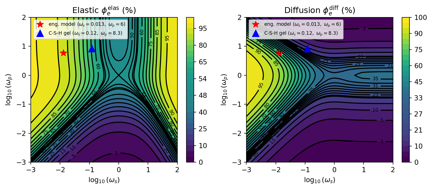
The 3D surfaces below are interactive: rotate, zoom and inspect values with the mouse.
fig_e = go.Figure(data=[go.Surface(
    z=Ze, x=logwp, y=logws,
    colorscale='RdBu_r',
    colorbar=dict(title='φ_e (%)'),
)])
fig_e.update_layout(
    title=dict(text='Elastic percolation threshold '
               'φ<sub>e</sub><sup>elas</sup> (%)'),
    scene=dict(
        xaxis_title='log₁₀(ωp)',
        yaxis_title='log₁₀(ωs)',
        zaxis_title='φe (%)',
        camera=dict(eye=dict(x=1.5, y=-1.5, z=1.2)),
    ),
    width=700, height=520,
    margin=dict(l=0, r=0, t=40, b=0),
)
fig_e.show()
fig_d = go.Figure(data=[go.Surface(
z=Zd, x=logwp, y=logws,
colorscale='RdBu_r',
colorbar=dict(title='φ_e (%)'),
)])
fig_d.update_layout(
title=dict(text='Diffusion percolation threshold '
'φ<sub>e</sub><sup>diff</sup> (%)'),
scene=dict(
xaxis_title='log₁₀(ωp)',
yaxis_title='log₁₀(ωs)',
zaxis_title='φe (%)',
camera=dict(eye=dict(x=1.5, y=-1.5, z=1.2)),
),
width=700, height=520,
margin=dict(l=0, r=0, t=40, b=0),
)
fig_d.show()The diagrams confirm the calibration rationale: with oblate solid (\(\omega_s \ll 1\)) and prolate pores (\(\omega_p \gg 1\)), the elastic and diffusion percolation thresholds are well separated — the solid skeleton percolates at high porosity (early hydration, low \(\alpha\)) while the pore network remains connected until very low porosity (late hydration). The engineering model calibration point (\(\omega_s = 0.013\), \(\omega_p = 6\), marked by \(\star\)) sits in a region where \(\phi_e^{\rm elas} \approx 15\,\%\) and \(\phi_e^{\rm diff} \approx 50\,\%\), consistent with reported setting degrees and with the experimentally observed diffusivity drop at intermediate to high hydration (Achour et al., 2020).
\(\,\)